Linear regression in R

library(tidyverse)
library(openintro)

`lm()` function

The function that will obtain the coefficients for the least-squares line is the lm() function. The syntax is as follows:

lm(response ~ explanatory, data)

Example: `elmhurst` data

Let’s once again consider the elmhurst data from openintro, where we want to fit the model

\[\text{gift aid} = \beta_{0} + \beta_{1} \times \text{income} + \epsilon\]

What does this look like in R?

lm(gift_aid ~ family_income, data = elmhurst)

Note that the variables have to be spelled as they appear in the data frame!

The output from this line of code is:


Call:
lm(formula = gift_aid ~ family_income, data = elmhurst)

Coefficients:
  (Intercept)  family_income  
     24.31933       -0.04307

This isn’t the most informative of output, so what we will do is use an additional function called summary() that will give us much more information!

We will first store the output from lm() as a variable called elmhurst_lm:

elmhurst_lm <- lm(gift_aid ~ family_income, data = elmhurst)

Then we will use the summary() function and pass in the linear model:

summary(elmhurst_lm)


Call:
lm(formula = gift_aid ~ family_income, data = elmhurst)

Residuals:
     Min       1Q   Median       3Q      Max 
-10.1128  -3.6234  -0.2161   3.1587  11.5707 

Coefficients:
              Estimate Std. Error t value             Pr(>|t|)    
(Intercept)   24.31933    1.29145  18.831 < 0.0000000000000002 ***
family_income -0.04307    0.01081  -3.985             0.000229 ***
---
Signif. codes:  0 '***' 0.001 '**' 0.01 '*' 0.05 '.' 0.1 ' ' 1

Residual standard error: 4.783 on 48 degrees of freedom
Multiple R-squared:  0.2486,    Adjusted R-squared:  0.2329 
F-statistic: 15.88 on 1 and 48 DF,  p-value: 0.0002289

There’s a lot more information here! We can now see the \(b_{0}\) and \(b_{1}\) estimates, along with some extra information. In particular, the “Multiple R-squared” quantity is the coefficient of determination \(R^2\)!

Sometimes we just want the coefficients. The coef() function will output the coefficients as a vector. These can be nice for reproducibility and in-line code:

coef(elmhurst_lm)

  (Intercept) family_income 
  24.31932901   -0.04307165

Pretty output using `broom`

The broom package has a function that turns the output from lm() into tidy, data frame form. We simply pass in the fitted model into the function of interest!

Install the package broom in the Packages pane!

`tidy()`

The function tidy() turns the information about the coefficients into a nice data frame:

library(broom)
tidy(elmhurst_lm)

# A tibble: 2 × 5
  term          estimate std.error statistic  p.value
  <chr>            <dbl>     <dbl>     <dbl>    <dbl>
1 (Intercept)    24.3       1.29       18.8  8.28e-24
2 family_income  -0.0431    0.0108     -3.98 2.29e- 4

Since this is in data frame form, each column is a variable, and all of our dplyr wrangling functions work!

tidy(elmhurst_lm) |>
  pull(estimate)

[1] 24.31932901 -0.04307165

`glance()`

The function glance() turns the extra information about the model fit into nice data frame:

glance(elmhurst_lm)

# A tibble: 1 × 12
  r.squared adj.r.squared sigma statistic  p.value    df logLik   AIC   BIC
      <dbl>         <dbl> <dbl>     <dbl>    <dbl> <dbl>  <dbl> <dbl> <dbl>
1     0.249         0.233  4.78      15.9 0.000229     1  -148.  302.  308.
# ℹ 3 more variables: deviance <dbl>, df.residual <int>, nobs <int>

glance(elmhurst_lm) |>
  pull(r.squared)

[1] 0.2485582

`augment()`

The function augment() takes a fitted SLR model input, and combines the x and y variables from the original data frame (i.e. family_income and gift_aid) with extra variables whose values come from the model fit

augment(elmhurst_lm) |>
  slice(1:3)

# A tibble: 3 × 8
  gift_aid family_income .fitted .resid   .hat .sigma  .cooksd .std.resid
     <dbl>         <dbl>   <dbl>  <dbl>  <dbl>  <dbl>    <dbl>      <dbl>
1     21.7         92.9     20.3   1.40 0.0204   4.83 0.000915      0.296
2     27.5          0.25    24.3   3.16 0.0727   4.81 0.0185        0.686
3     27.8         53.1     22.0   5.72 0.0321   4.76 0.0245        1.22

You can see we have the new variables:

.fitted: the fitted (estimated) values \(\hat{y}\) for the corresponding observation
.resid: the residual for the observation

The periods are important!

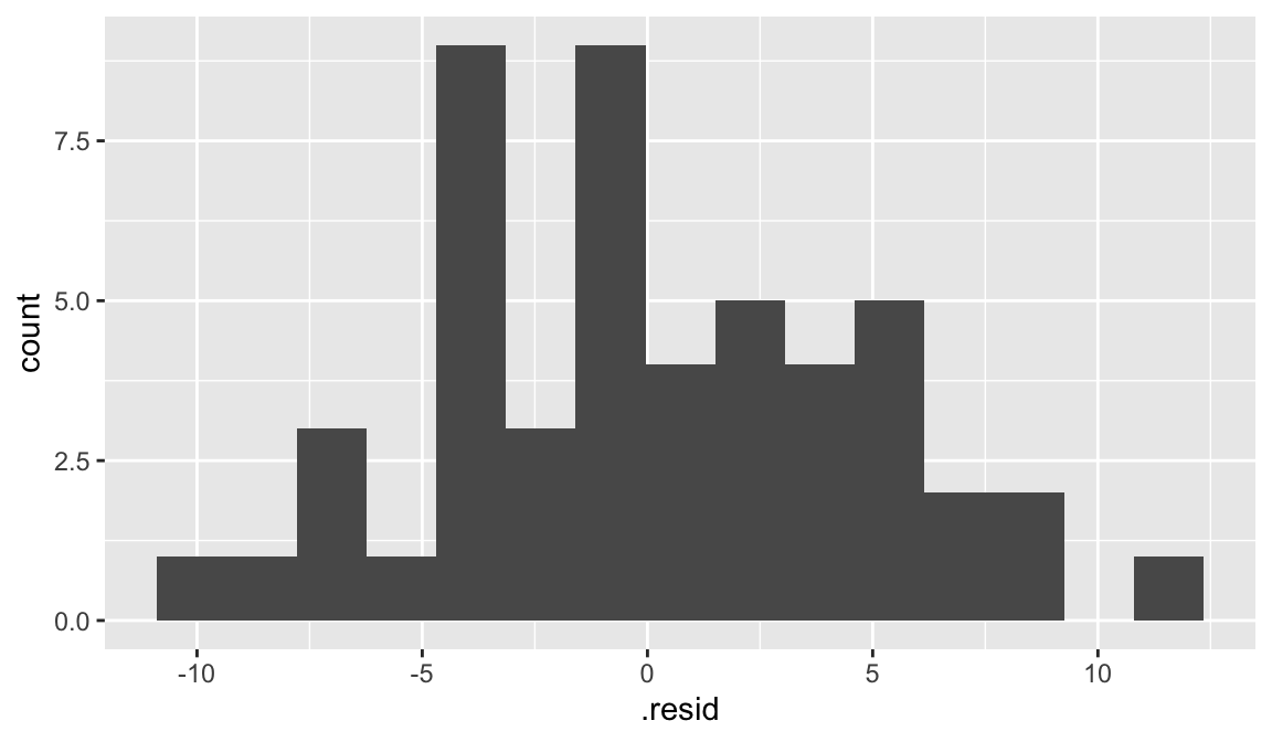
We can use the output from augment to plot histogram of residuals:

augment(elmhurst_lm) |>
  ggplot(aes(x = .resid)) +
  geom_histogram(bins = 15)

lm() function

Example: elmhurst data

Pretty output using broom

tidy()