Numerical data

Visualization and summary statistics (part 1)

2025-09-15

Housekeeping

• Where to find feedback on coding practice
• Problem set 1 due tonight!
• Office hours today 2-3pm
• Activity!

Variables types

• Variables can be broadly broken into two categories: numerical (quantitative) or categorical (qualitative)

• Numerical variables take a wide range of numerical values, and it is sensible to add/subtract/do mathematical operations with those values. Two types:

  1. Discrete if it can only take on finitely many numerical values within a given interval

  2. Continuous if it can take on any infinitely many values within a given interval

• Categorical variables are essentially everything else (more on this next week!)

• Examples and non-examples?

Example

We will be looking at some medical insurance data throughout these slides.

Which of the following variables are numerical? Which are discrete vs. continuous?

Summary statistics for numerical data

Condensing information

• We often care about variable’s distribution: the different values the variable can take on along with how often

• Rather than provide someone with an entire dataset, it is more useful to provide quick “snapshot” information

• Two pieces of quantitative information that describe a distribution:

  • Center

  • Spread

Mean

• Most common way to measure the center of the distribution of a numerical variable is using the mean (also called the average)

• Sample mean: a mean calculated using sampled data. The sample mean is typically denoted as \(\bar{x}\)

  • \(x\) is a placeholder for the variable of interest (e.g. BMI, charges)
  • The bar communicates that we are looking at the average

• The sample mean is the sum over all the observed values of the variable, divided by total number of observations \(n\):

\[\bar{x} = \frac{x_{1} + x_{2} + \ldots x_{n}}{n} = \frac{1}{n} \sum_{i=1}^{n} x_{i}\]

Mean (cont.)

• The sample mean \(\bar{x}\) is an example of a sample statistic

• The mean over the entire population is an example of a population parameter. The population mean is denoted \(\mu\) (Greek letter mu)

  • The sample mean \(\bar{x}\) is often used as an estimate for \(\mu\) (more on this in a few weeks!)

Examples

• Let’s calculate the sample mean weight of a piece of candy in our bag. Let \(x\) be the weight of a candy.

  • Calculate your \(\bar{x}\)

• How would we obtain the population mean \(\mu\)?

• What is the average of the following values? \(\qquad 1, 4, 4\)

• If instead there were ten 1’s and twenty 4’s, would the average be the same?

• Thus, we see that means depend on proportions!

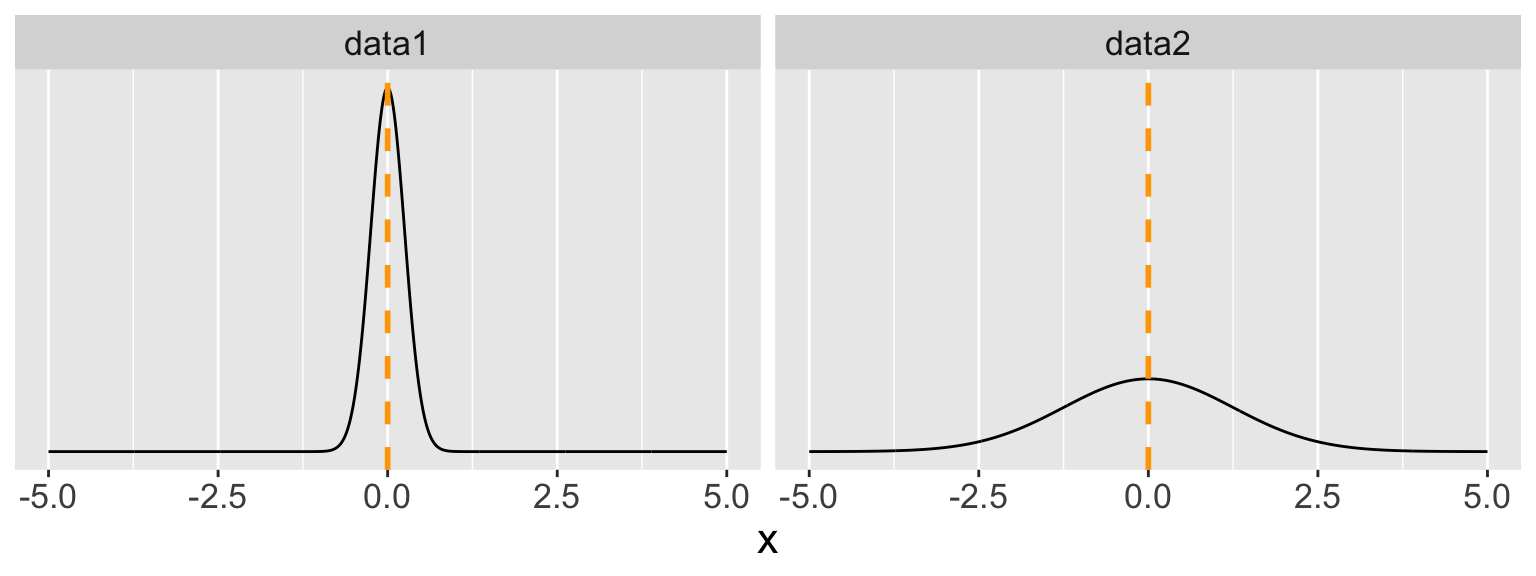
Variability

• At the heart of statistics is also the variability or spread of the distribution of the variable

• We will work with variance and standard deviation, which are ways to describe how spread out data are from their mean

Deviation

We begin with deviation, which is the distance or difference between an observation from the (sample) mean

• How might we write this using statistical notation?
• Let’s write out the deviations of your five sampled weights

Variance and standard deviation

• The sample variance \(s^2\) squares the deviations and takes an average:

  \[ s^2 = \frac{1}{n-1}\sum_{i=1}^{n} (x_{i} - \bar{x})^2 \]

  • Let’s talk about this notation and intuition behind this formula. In particular, there are at least two things to note

• Set-up the calculation of the sample variance of your sample

  • I will calculate this in R

• The sample standard deviation \(s\) is the simply the square root of the sample variance (\(s = \sqrt{s^2}\))

Variance and standard deviation (cont.)

• Like the mean, the population values for variance and standard deviation are denoted with Greek letters:

  • \(\sigma\) for population standard deviation (Greek letter “sigma”)

  • \(\sigma^2\) for population variance

• If the calculation of standard deviation is a more complicated quantity than the variance, why do we bother with standard deviation?

Live code

Functions to calculate sample mean, variance, and standard deviation in R. Each expects a vector of numerical values as input:

• mean()

• var()

• sd()

Visualizing numerical data

Scatterplots

Scatterplots are bivariate (two-variable) visualizations that provide a case-by-case view of the data for two numerical variables

• Each point represents the observed pair of values of variables 1 and 2 for a case in the dataset

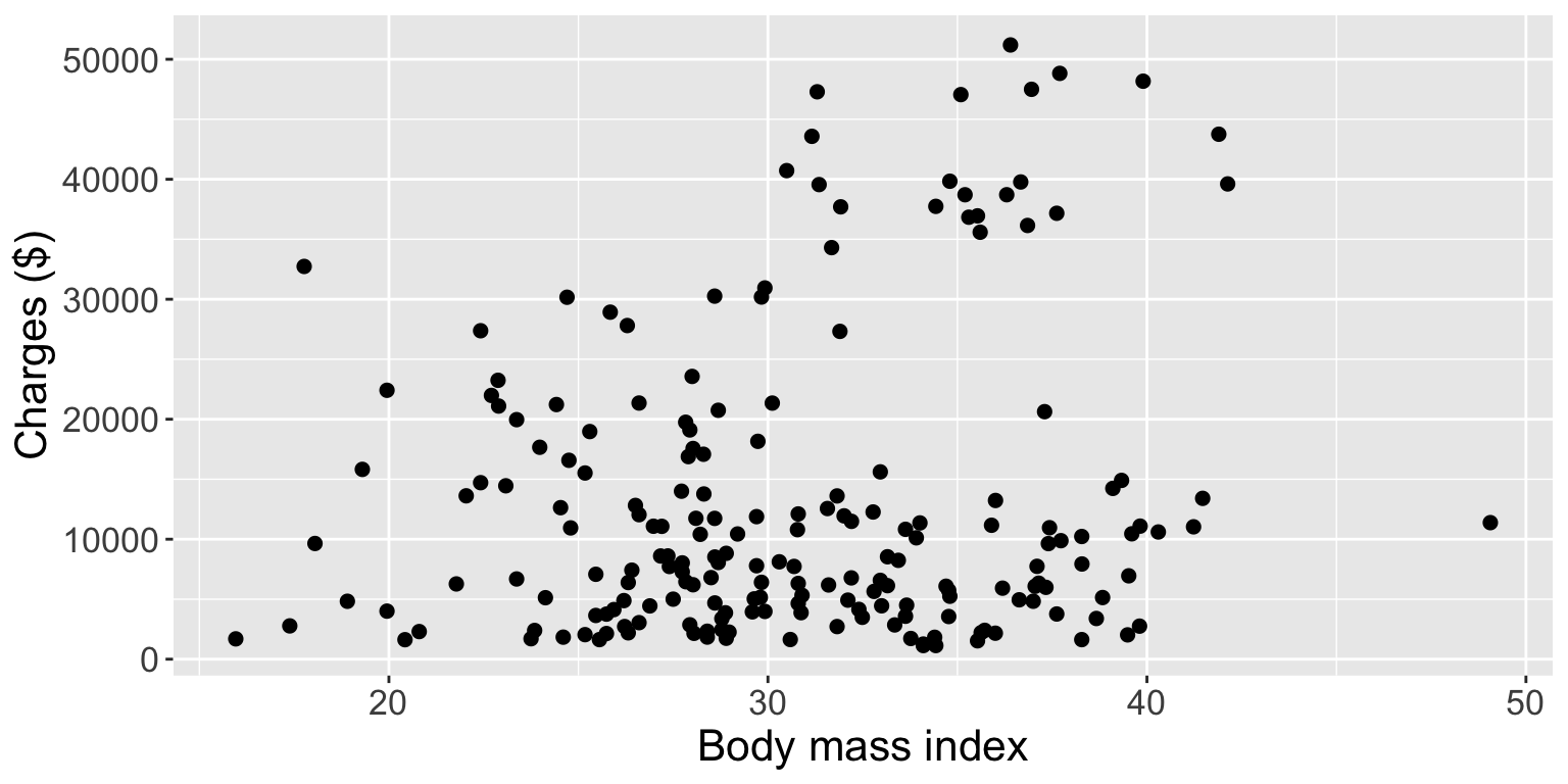
Scatterplots (cont.)

Use scatterplots to reveal:

• Association (positive, negative, none), and if there is an association:

  • The strength (very weak to very strong)

  • The type of association (e.g. linear, quadratic)

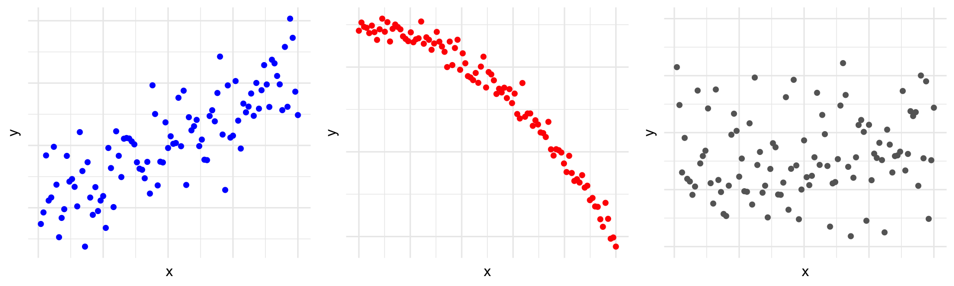
• If there is a notion of explanatory and response, the explanatory goes on \(x\)-axis!

Visualizing univariate numerical data

• To visualize the distribution (i.e. behavior) of a single variable, we could create a dot plot where:

  • Each case is plotted on a horizontal axis as a dot

  • Values that appear multiple times in the dataset would have stacked dots

• We can make a dot plot from our activity

• Pros and cons?

Binning

• We will sacrifice precision for convenience by binning:
  • Segment the variable into equal-sized bins
  • Visualize the value of each observation using its corresponding bin
• For example, the bmi variable has observed values of \(15.96\) through \(49.6\). Consider the following bins of size 5: [15, 19), [19, 23), [23, 27), …, [49, 53)
  • Convention of left or right inclusive?
• We tabulate/count up the number of observations that fall into each bin.

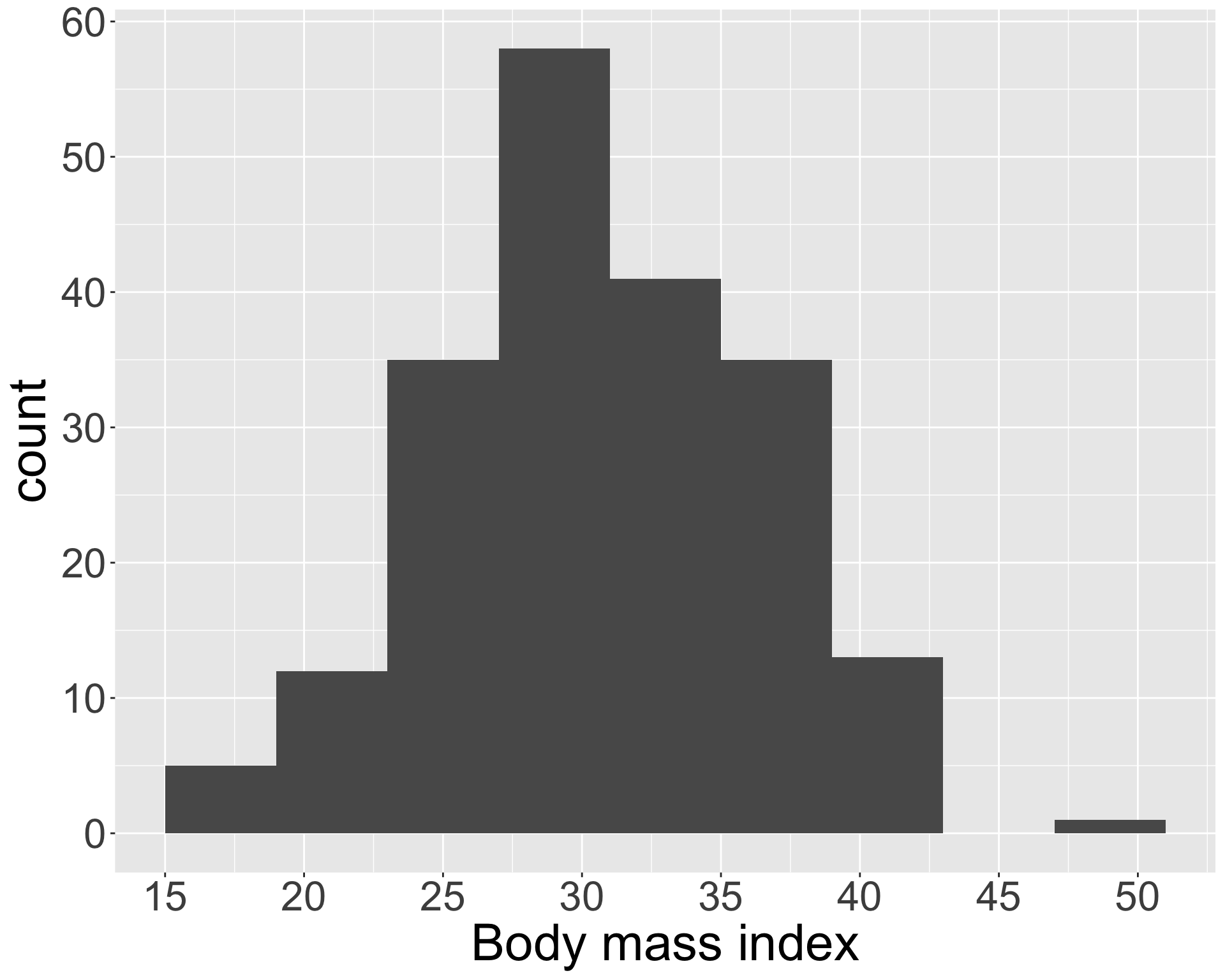
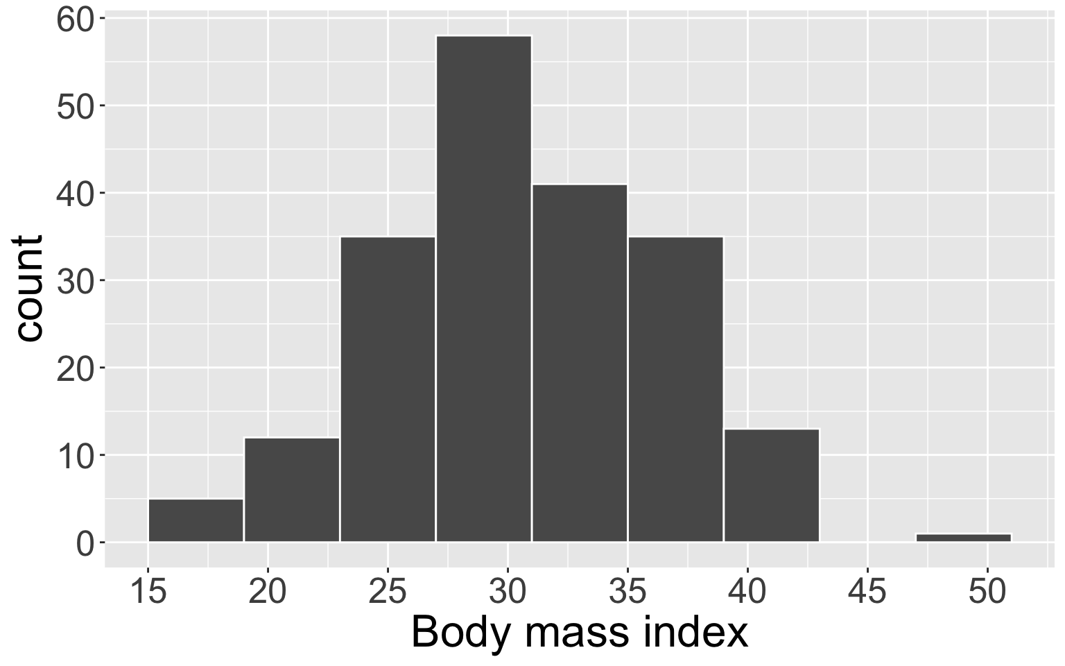
Histograms

Histograms are visualizations that display the binned counts as bars for each bin.

• Histograms provide a view of the density of the data (the values the data take on as well as how often)

bmi_bin	count
[15, 19)	5
[19, 23)	12
[23, 27)	35
[27, 31)	58
[31, 35)	41
[35, 39)	35
[39, 43)	13
[49, 52)	1

Describing distributions

A convenient way to describe a variable’s behavior is through the shape of its distribution. Using histograms, we should identify:

1. Skewness (or lack thereof):
   • Distributions with long tails to the left are called left-skewed
   • Distributions with long tails to the right are right-skewed
   • If not skewed, then the distribution is symmetric
2. Modes: prominent peaks in the distribution
   • Distribution may be unimodal (one peak), bimodal (two peaks), or multimodal (more than two peaks)
   • Peaks need not be same height

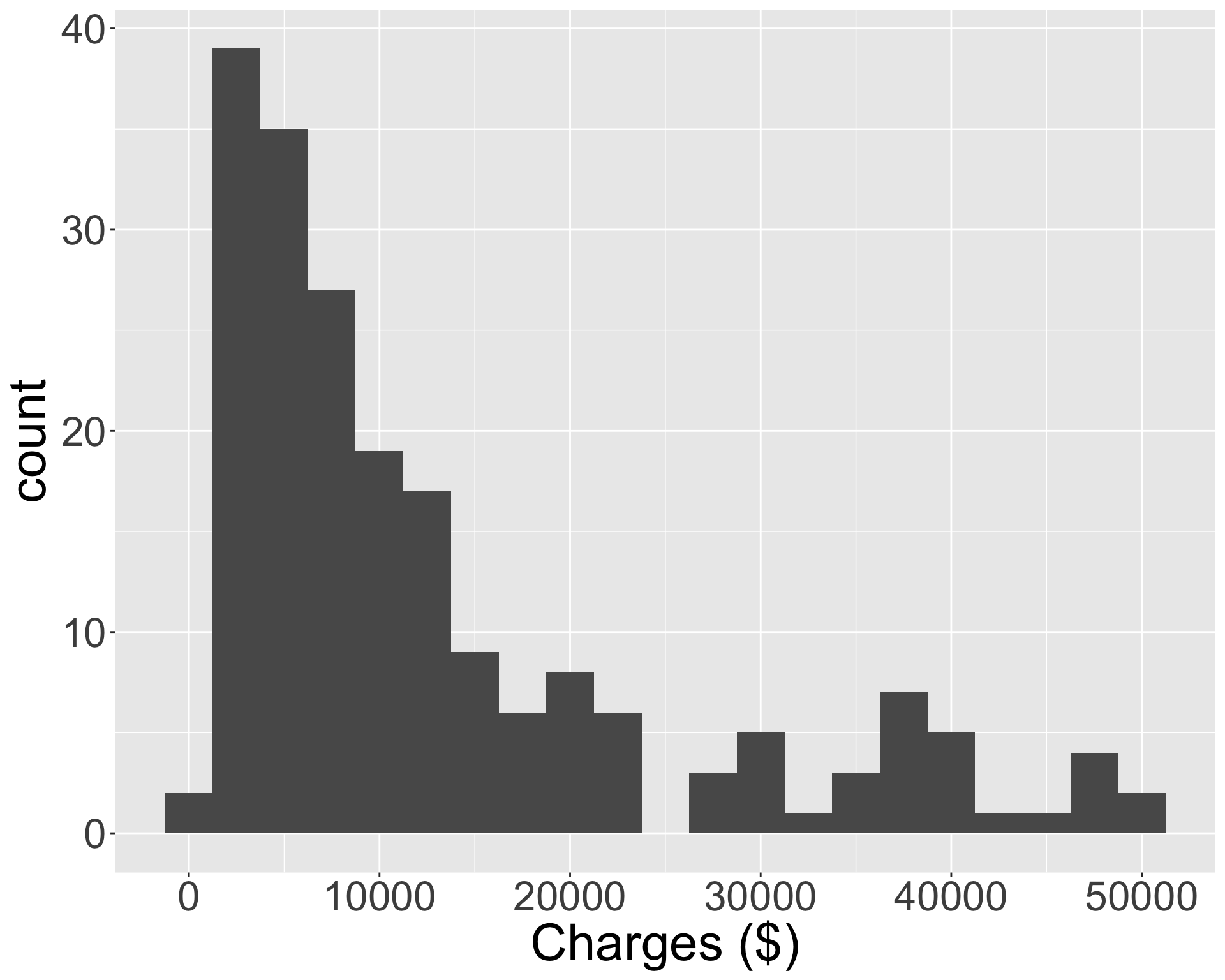
Histograms (cont.)

How would you describe the shape (i.e. skewness and modality) of the distributions in the following two histograms?

Creating visualizations

Working in your groups:

1. Using a histogram, visualize the distribution of the sample mean weights from our activity
2. Convince yourselves as a group: what does a case represent in this data?
3. Describe the shape of your distribution (i.e. skewness and modality)
4. Obtain the sample mean and standard deviation of the sample means