Visualizations with ggplot

2025-09-18

Exploratory data analysis

• Exploratory data analysis (EDA) is an approach to analyzing data sets to summarize the main characteristics.

  • Often visual through plots

• Because of its name “exploratory”, we typically perform EDA at the beginning of a project

• Can also calculate summary statistics and perform data wrangling/manipulation/transformation at (or before) this stage of the analysis

Tidy data

• When working with data in R, always look at the data to ensure it is in tidy format:

  • Each row represents an observation, each column represents a variable describing the observations

• anscombe data frame: four datasets each with 11 observations each and the same two variables x and y

Non-tidy version:

   x1 x2 x3 x4    y1   y2    y3    y4
1  10 10 10  8  8.04 9.14  7.46  6.58
2   8  8  8  8  6.95 8.14  6.77  5.76
3  13 13 13  8  7.58 8.74 12.74  7.71
4   9  9  9  8  8.81 8.77  7.11  8.84
5  11 11 11  8  8.33 9.26  7.81  8.47
6  14 14 14  8  9.96 8.10  8.84  7.04
7   6  6  6  8  7.24 6.13  6.08  5.25
8   4  4  4 19  4.26 3.10  5.39 12.50
9  12 12 12  8 10.84 9.13  8.15  5.56
10  7  7  7  8  4.82 7.26  6.42  7.91
11  5  5  5  8  5.68 4.74  5.73  6.89

Tidy version (first 15 rows):

   set  x     y
1    I 10  8.04
2    I  8  6.95
3    I 13  7.58
4    I  9  8.81
5    I 11  8.33
6    I 14  9.96
7    I  6  7.24
8    I  4  4.26
9    I 12 10.84
10   I  7  4.82
11   I  5  5.68
12  II 10  9.14
13  II  8  8.14
14  II 13  8.74
15  II  9  8.77

Data visualization

• Data visualization is the creation and study of the visual representation of data

• We have learned how to use base R code to make simple histograms. We will now use ggplot2 which makes customization easier

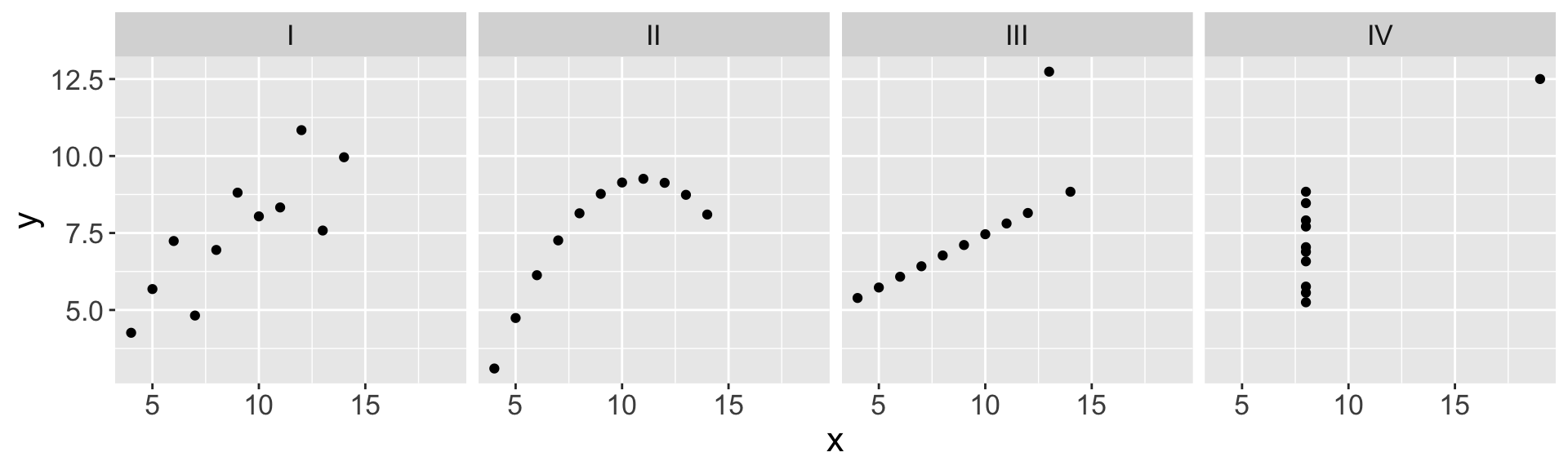
Why do we visualize?

• Summary statistics from each of the four datasets in anscombe:

# A tibble: 4 × 5
  set   mean_x mean_y  sd_x  sd_y
  <fct>  <dbl>  <dbl> <dbl> <dbl>
1 I          9   7.50  3.32  2.03
2 II         9   7.50  3.32  2.03
3 III        9   7.5   3.32  2.03
4 IV         9   7.50  3.32  2.03

• Let’s visualize the four data sets. What would be an appropriate type of plot to examine the relationship between the two quantitative variables x and y?

Introduction to ggplot

• We will learn how to create histograms, box plots, and scatterplots using the ggplot() function from the ggplot2 library (included in tidyverse)

  • Plots are constructed in layers

• At a minimum, we need to specify 1) the dataset, 2) variable(s) from the dataset we’d like to plot, and 3) the type of plot

  • How does this differ from the previous coding practice?

• This is what the code will generally look like. Values in < > and xxx denote what you as the coder need to specify.

ggplot(data = <dataset>, # specify data frame
       mapping = aes(x = <x-var>)) + #  specify variables to be used in plot
  geom_xxx() + # specify plot type
  <other options>

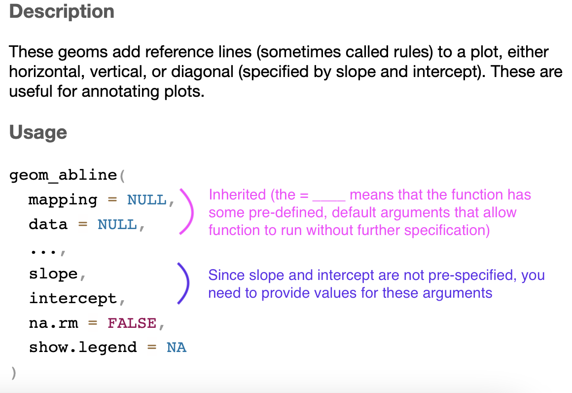
Inheriting arguments

• Many functions related to plotting in ggplot take the form geom_xxx()

• The Help file for these functions show that the first two arguments are mapping and data. These are automatically inherited from the mapping and data arguments in the first layer ggplot() function

  • i.e. you don’t need to re-specify them, unless you are trying to add a new data frame’s data to your visualization

Additional variables + modifications

• We emphasize making informative and useful visualizations.

  • Informative titles and labels

  • Plot should tell a meaningful story

• Depending on the plot and data, we can map additional variables by:

  1. Specifying visual cues via aesthetics: color, size, shape, alpha (transparency)

  2. Faceting (will see this next week)

Live code

Note: most of the code I will show is included in the remaining slides. However, we will most likely go off-script based on questions from the class!

Slides on ggplot()

geom_histogram()

ggplot(data = insurance,  mapping = aes(x = charges)) +
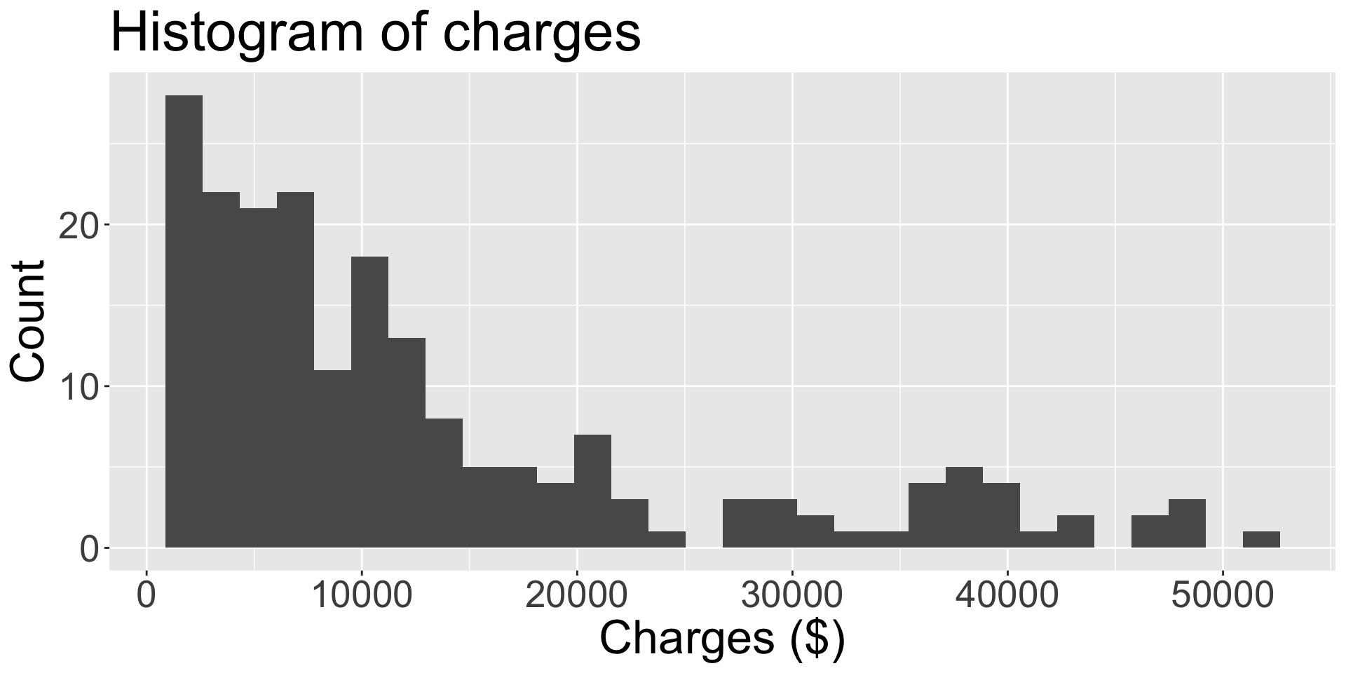
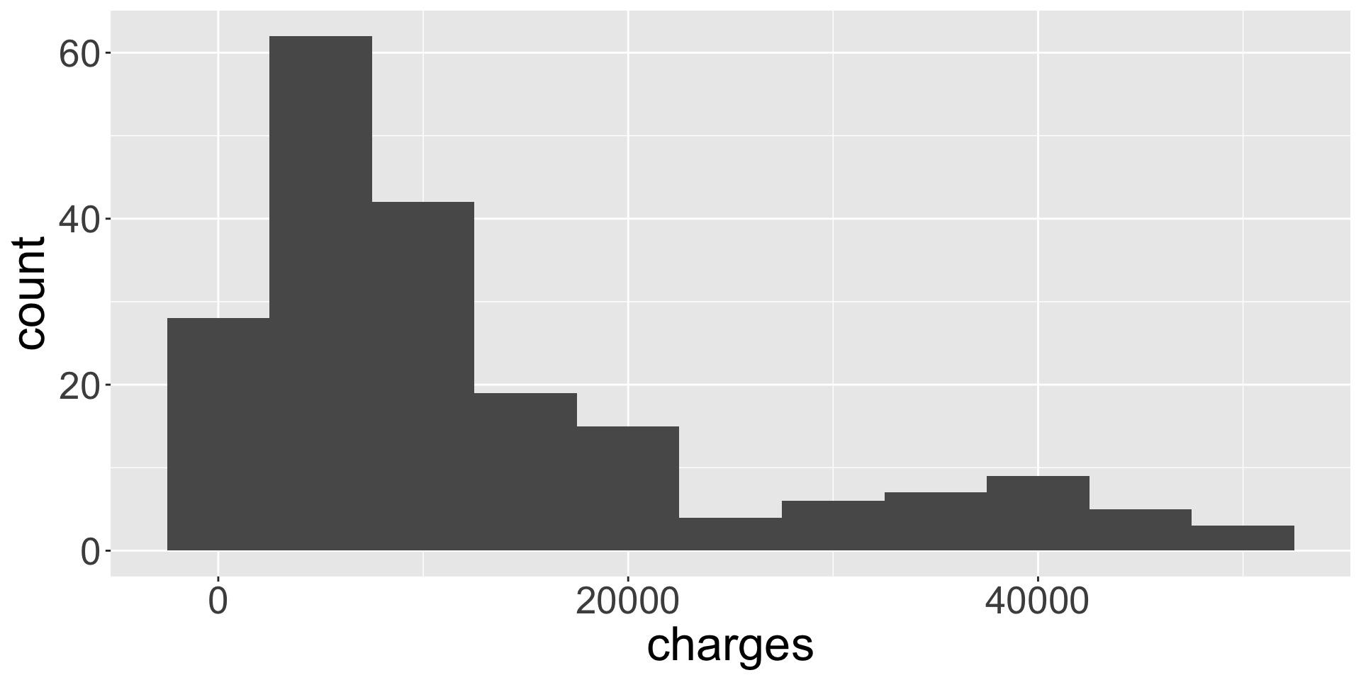
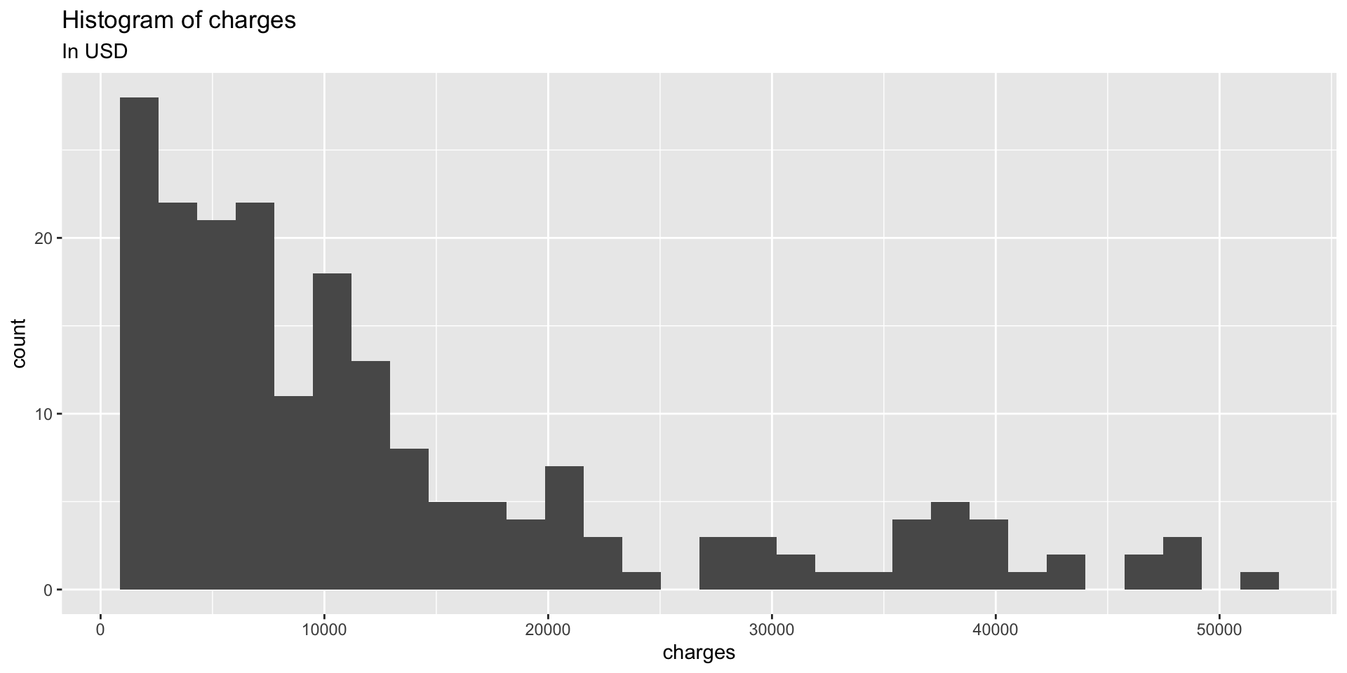
  geom_histogram()

`stat_bin()` using `bins = 30`. Pick better value with `binwidth`.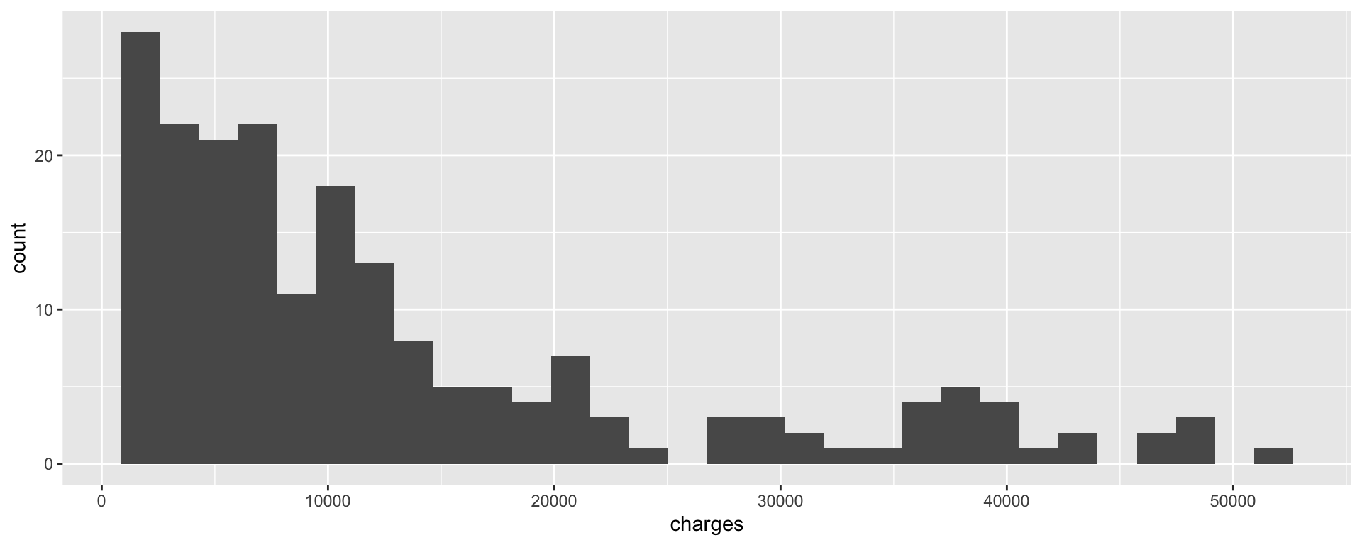

Note the message provided when you execute this code!

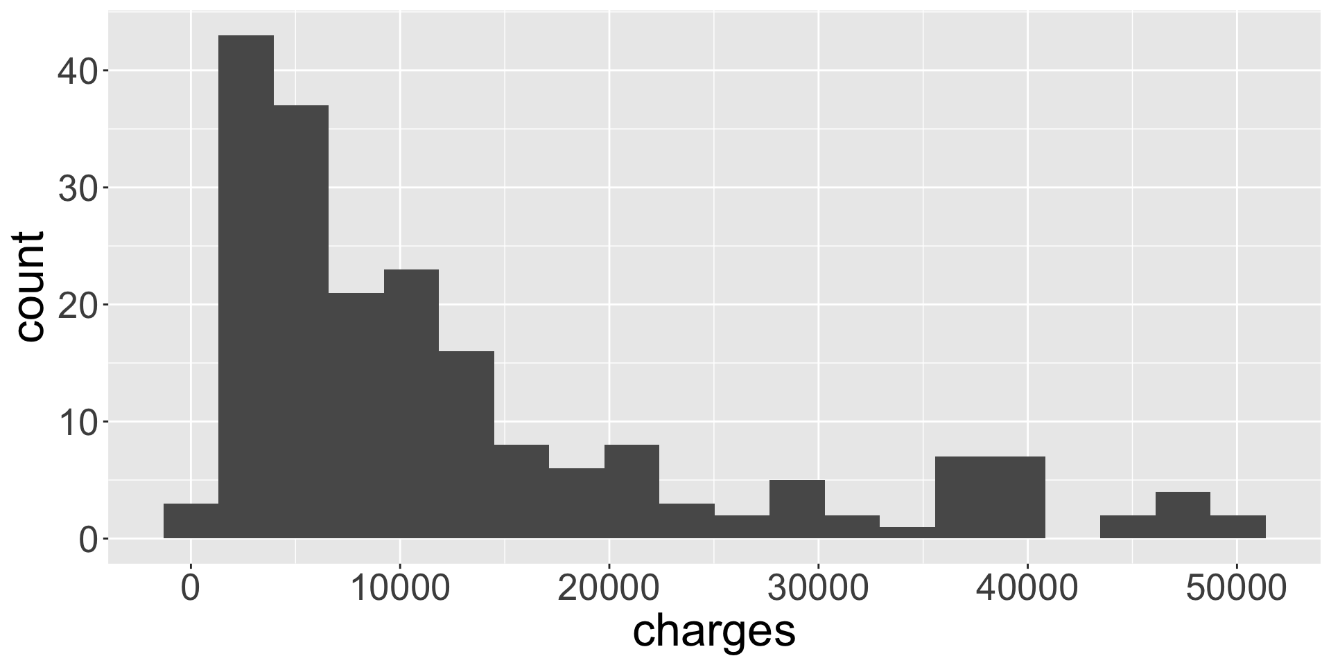
geom_histogram() cont.

To improve on histogram we change the bin width.

ggplot(data = insurance, 
       mapping = aes(x = charges)) +
  geom_histogram(binwidth = 5000)

ggplot(data = insurance, 
       mapping = aes(x = charges)) +
  geom_histogram(bins = 20)

geom_boxplot()

ggplot(data = insurance, mapping = aes(x = charges)) +
  geom_boxplot()

ggplot(data = insurance, 
       mapping = aes(y = charges)) +
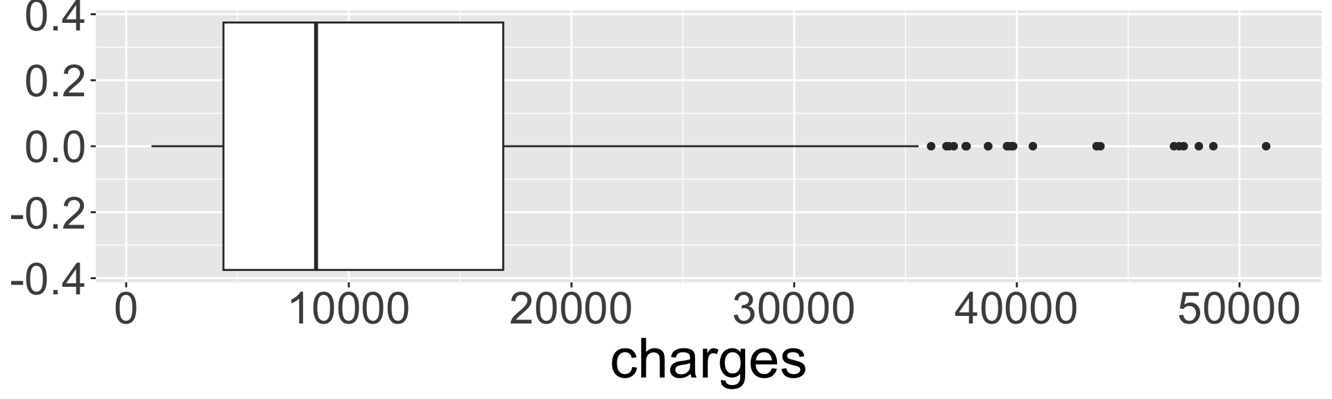
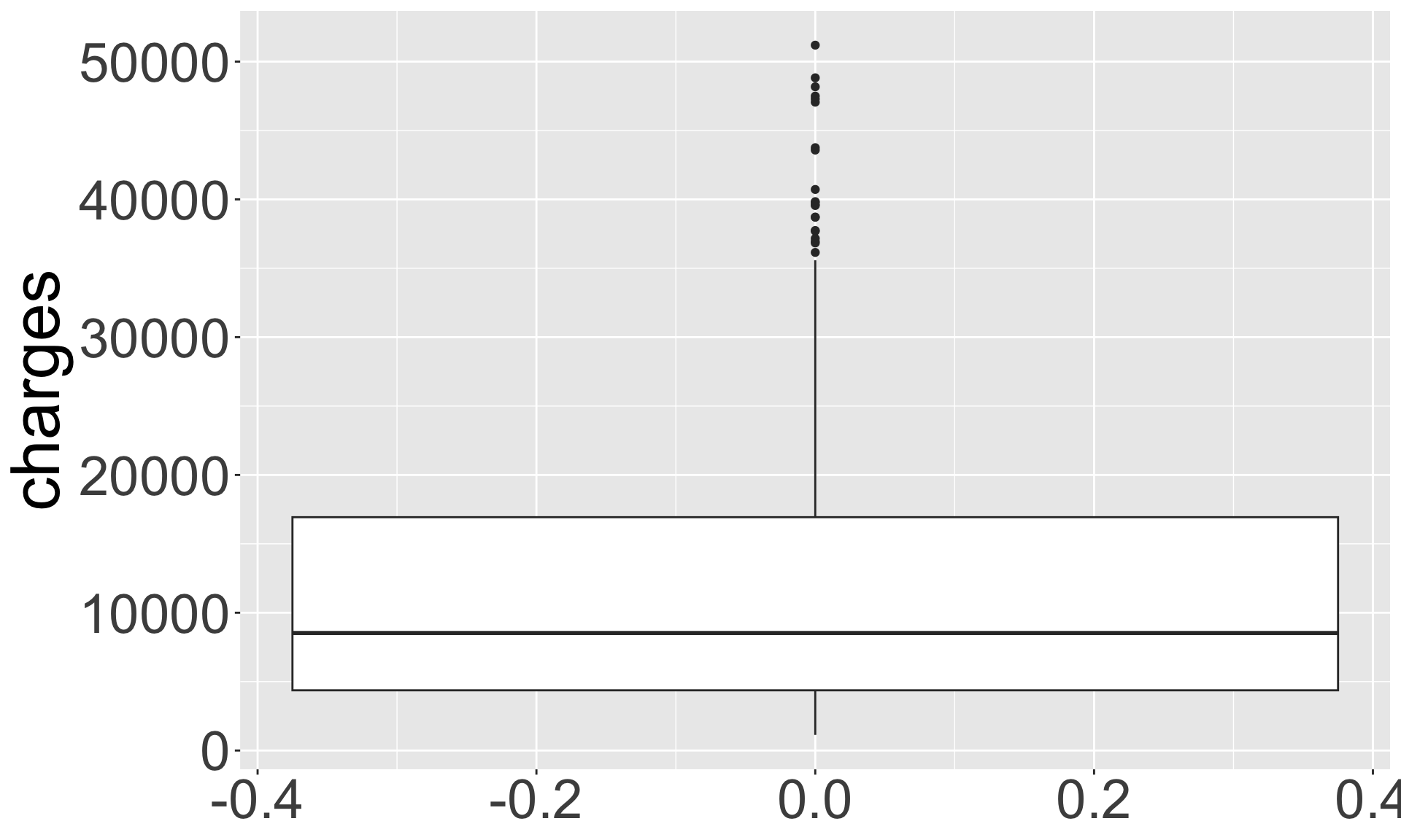
  geom_boxplot()

geom_point()

ggplot(data = insurance, mapping = aes(x = age, y = charges)) +
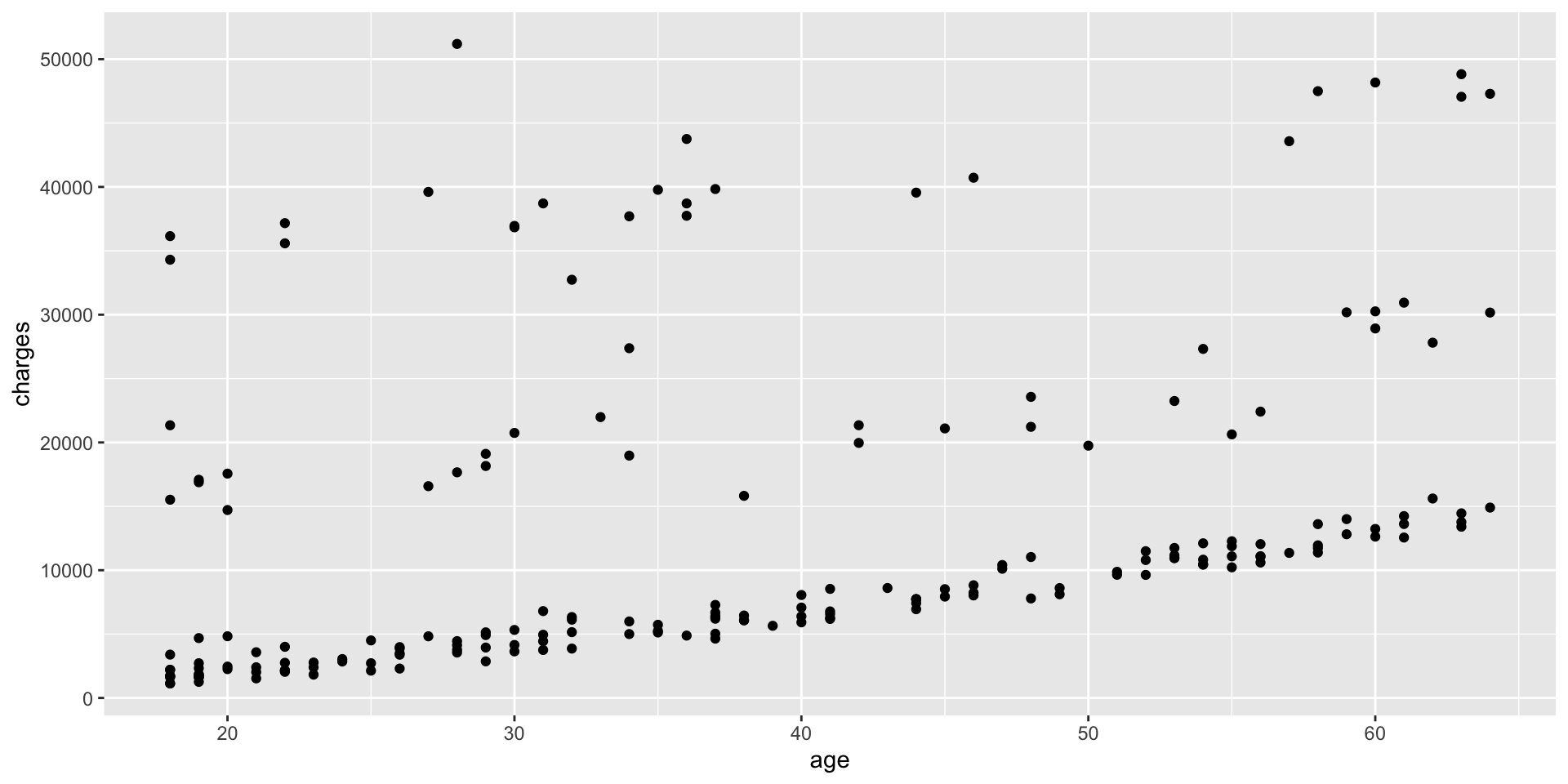
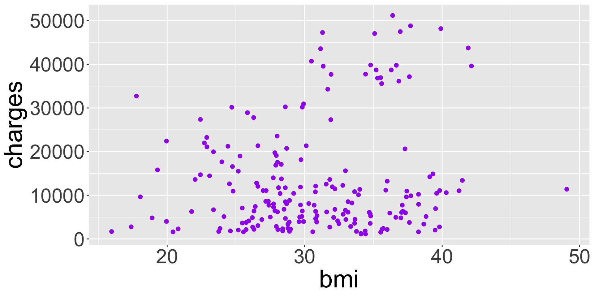
  geom_point()

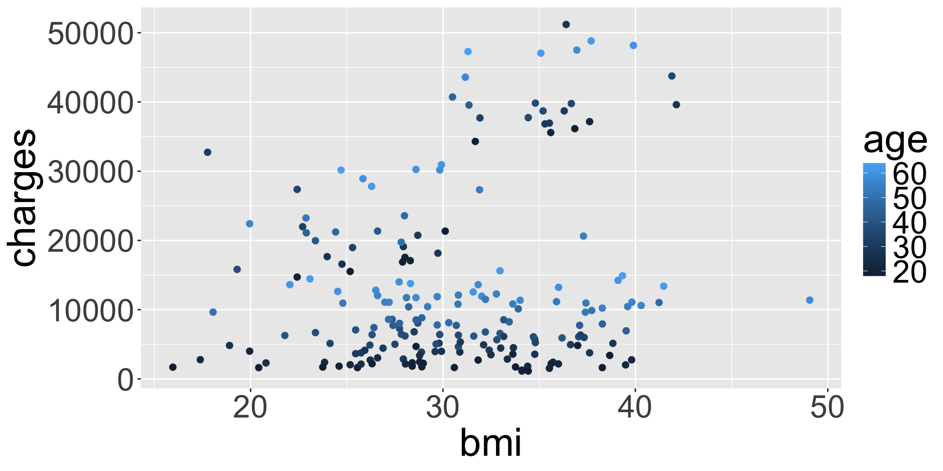
Aesthetics: color

ggplot(data = insurance, 
       mapping = aes(x = bmi, y = charges, 
                     col = age)) +
  geom_point()

ggplot(data = insurance, 
       mapping = aes(x = bmi, y = charges)) +
  geom_point(aes(col = age))

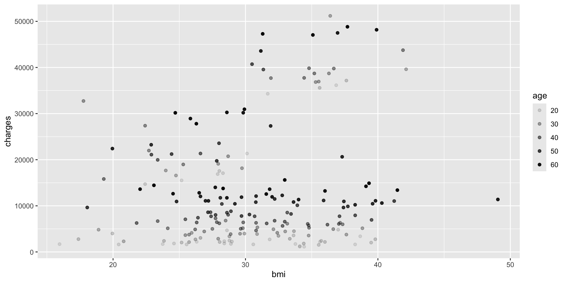
Aesthetics: transparency

ggplot(data = insurance, mapping = aes(x = bmi, y = charges, 
                                       alpha = age)) +
  geom_point()

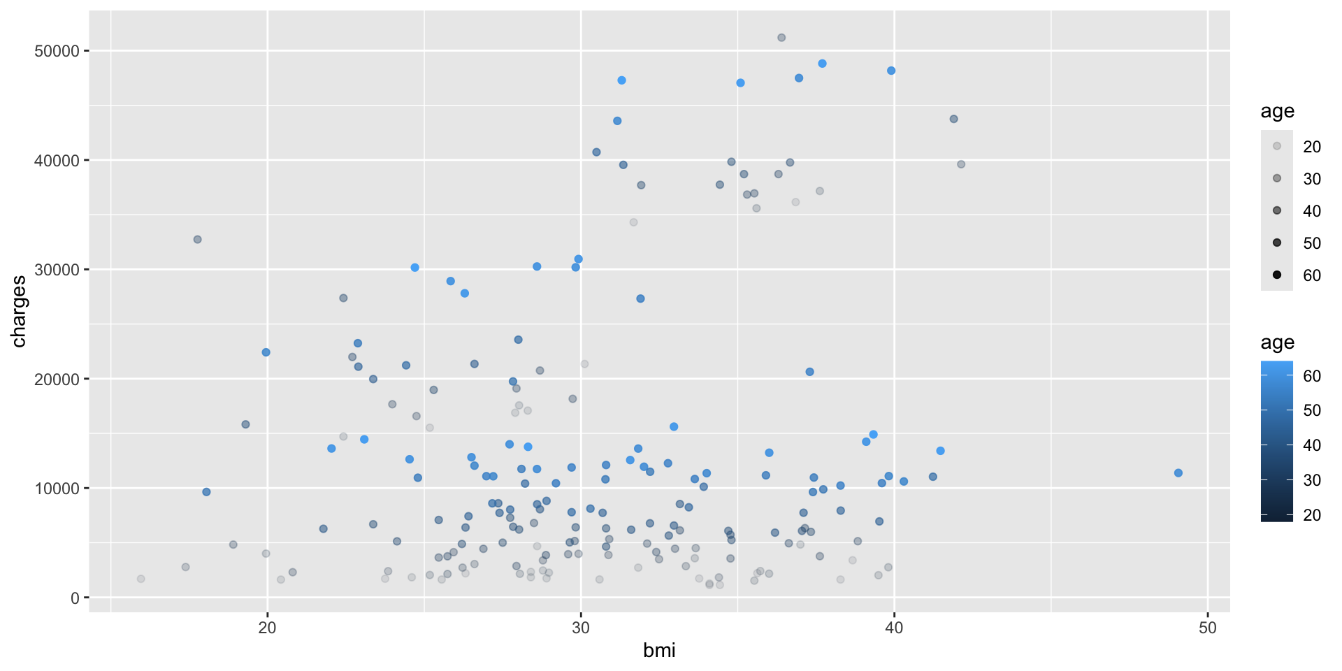
Specifying multiple aesthetics

ggplot(data = insurance, mapping = aes(x = bmi, y = charges, col = age, alpha = age)) +
  geom_point()

When to map to variable

What’s going on here?

ggplot(data = insurance, 
       mapping = aes(x = bmi, y = charges)) +
  geom_point(col = "purple")

ggplot(data = insurance, 
       mapping = aes(x = bmi, y = charges)) +
  geom_point(aes(col = "purple"))

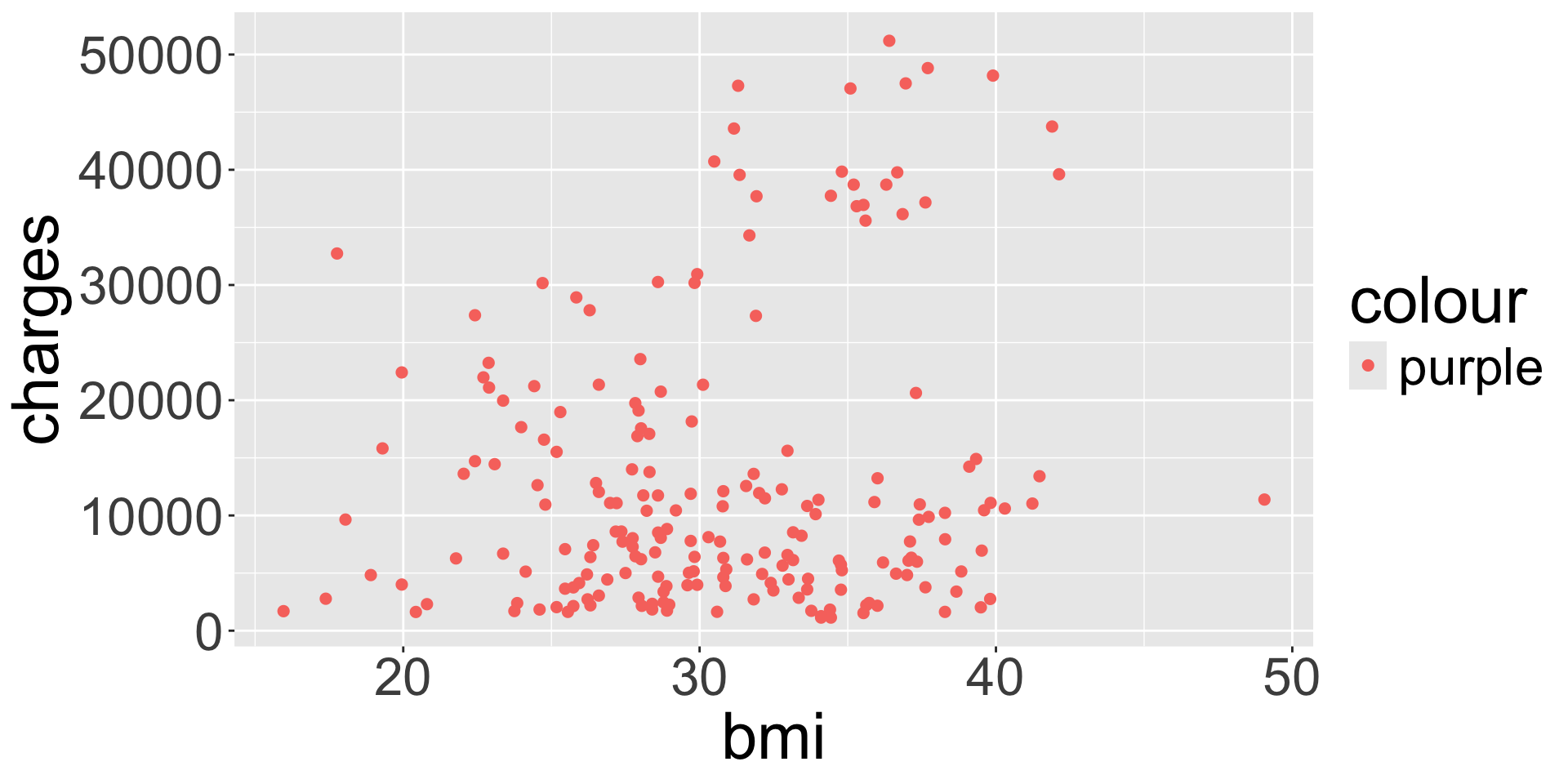
• Key takeaway: aesthetics should correspond/map to a variable in the data frame

  • “Fixed” visual cues are set outside of aes()

Adding a title

ggplot(data = insurance, mapping = aes(x = charges)) +
  geom_histogram() +
  ggtitle("Histogram of charges",
          subtitle = "In USD")

Changing axis labels

By default, axis titles are taken from variable name specified in aes(). To change:

ggplot(data = insurance, 
       mapping = aes(x = charges)) +
  geom_histogram() +
  ggtitle("Histogram of charges") +
  xlab("Charges ($)")

ggplot(data = insurance, 
       mapping = aes(x = charges)) +
  geom_histogram() +
  labs(title = "Histogram of charges",
       x = "Charges ($)", y = "Count")