Joins data frames and pivoting

2025-12-01

Housekeeping

Content today is optional; might be useful for your final project!

Pivoting

Wide data

Let’s take a look at first few observations of the relig_income data frame from tidyverse package:

relig_income |>
  head()

# A tibble: 6 × 11
  religion  `<$10k` `$10-20k` `$20-30k` `$30-40k` `$40-50k` `$50-75k` `$75-100k`
  <chr>       <dbl>     <dbl>     <dbl>     <dbl>     <dbl>     <dbl>      <dbl>
1 Agnostic       27        34        60        81        76       137        122
2 Atheist        12        27        37        52        35        70         73
3 Buddhist       27        21        30        34        33        58         62
4 Catholic      418       617       732       670       638      1116        949
5 Don’t kn…      15        14        15        11        10        35         21
6 Evangeli…     575       869      1064       982       881      1486        949
# ℹ 3 more variables: `$100-150k` <dbl>, `>150k` <dbl>,
#   `Don't know/refused` <dbl>

This data is currently in “wide” format: a row has more than one observation. That is, the same outcome variable appears in multiple columns.
- The outcome observation that spans across several columns is income range.
- The different incomes columns are essentially different levels of the same categorical variable.

Long data

We might want long format: the outcome variable only exists in one column, and a second column/variable tells us the different levels.

Each row has one observation, but the units of observation (in this case, number of people in each income bracket) are repeated down one column.
This is helpful for us to perform group_by() or facet_wrap().

Converting from wide -> long

We will do this with the pivot_longer() function. This function requires a couple of arguments:

cols: which columns to pivot into a “longer” format. That is, the columns that we should “move”
names_to: a string character that provides the new column name for the categorical variable you are creating
values_to: a string character that provides the new variable name for the response/outcome variable that is common across all levels of the categorical variable

relig_income |>
  pivot_longer(cols = 2:11, 
               names_to = "income_range",  
               values_to = "count")

pivot_longer()

Resulting data frame:

# A tibble: 20 × 3
   religion income_range       count
   <chr>    <chr>              <dbl>
 1 Agnostic <$10k                 27
 2 Agnostic $10-20k               34
 3 Agnostic $20-30k               60
 4 Agnostic $30-40k               81
 5 Agnostic $40-50k               76
 6 Agnostic $50-75k              137
 7 Agnostic $75-100k             122
 8 Agnostic $100-150k            109
 9 Agnostic >150k                 84
10 Agnostic Don't know/refused    96
11 Atheist  <$10k                 12
12 Atheist  $10-20k               27
13 Atheist  $20-30k               37
14 Atheist  $30-40k               52
15 Atheist  $40-50k               35
16 Atheist  $50-75k               70
17 Atheist  $75-100k              73
18 Atheist  $100-150k             59
19 Atheist  >150k                 74
20 Atheist  Don't know/refused    76

Note that the unit of observation is repeated down several rows!

# This also works
relig_income |>
  pivot_longer(cols = !religion, names_to = "income_range",  values_to = "count")

Converting long -> wide

Let’s look at the fish_encounters data. Convince yourself that it’s currently in long format!

# A tibble: 6 × 3
  fish  station  seen
  <fct> <fct>   <int>
1 4842  Release     1
2 4842  I80_1       1
3 4842  Lisbon      1
4 4842  Rstr        1
5 4842  Base_TD     1
6 4842  BCE         1

We want to pivot the data such that each fish is an observation, and we can easily see which stations it was observed at.
We can do this using the pivot_wider() function!

pivot_wider()

The pivot_wider() function takes two arguments:

names_from: the name of the variable(s) in the data frame to get the name of the output column.
values_from: the name of the variable(s) in the data frame to get the cell values from

The input to names_from should be the categorical variable(s), and the different levels of this categorical variable will be the new column names.
- What should we fill these cells with? The values specified by values_from.

fish_encounters |>
  pivot_wider(names_from = station, values_from = seen)

pivot_wider()

# A tibble: 19 × 12
   fish  Release I80_1 Lisbon  Rstr Base_TD   BCE   BCW  BCE2  BCW2   MAE   MAW
   <fct>   <int> <int>  <int> <int>   <int> <int> <int> <int> <int> <int> <int>
 1 4842        1     1      1     1       1     1     1     1     1     1     1
 2 4843        1     1      1     1       1     1     1     1     1     1     1
 3 4844        1     1      1     1       1     1     1     1     1     1     1
 4 4845        1     1      1     1       1    NA    NA    NA    NA    NA    NA
 5 4847        1     1      1    NA      NA    NA    NA    NA    NA    NA    NA
 6 4848        1     1      1     1      NA    NA    NA    NA    NA    NA    NA
 7 4849        1     1     NA    NA      NA    NA    NA    NA    NA    NA    NA
 8 4850        1     1     NA     1       1     1     1    NA    NA    NA    NA
 9 4851        1     1     NA    NA      NA    NA    NA    NA    NA    NA    NA
10 4854        1     1     NA    NA      NA    NA    NA    NA    NA    NA    NA
11 4855        1     1      1     1       1    NA    NA    NA    NA    NA    NA
12 4857        1     1      1     1       1     1     1     1     1    NA    NA
13 4858        1     1      1     1       1     1     1     1     1     1     1
14 4859        1     1      1     1       1    NA    NA    NA    NA    NA    NA
15 4861        1     1      1     1       1     1     1     1     1     1     1
16 4862        1     1      1     1       1     1     1     1     1    NA    NA
17 4863        1     1     NA    NA      NA    NA    NA    NA    NA    NA    NA
18 4864        1     1     NA    NA      NA    NA    NA    NA    NA    NA    NA
19 4865        1     1      1    NA      NA    NA    NA    NA    NA    NA    NA

Note that there are some NA values after pivoting. From the Help file, this is because misses were not directly recorded in the original form of the data. Try adding the argument values_fill = 0 to the pivot_wider() function.

Joins

Joining data frames

Assume we have two data frames, df1 and df2. There are some shared variable(s) across the two.

We want to combine df1 and df2 into one single data frame. The dplyr code will look something like:

xxx_join(df1, df2)

How do we combine df1 and df2 them? The following mutating joins give us rules:
- left_join(): keep all cases from df1
- right_join(): keep all cases from df2
- full_join(): keep all cases from both df1 and df2
- inner_join(): keep all cases from df1 where there are matching values in df2 (more complicated in the scenario of multiple matches)

I know this is confusing! Examples will help clarify!

Setup

For the next few slides…

df1

ID	name
1	x1
2	x2
3	x3

df2

ID	grade
1	y1
2	y2
4	y4

I recommend writing these two down, as we will work with them in the next few slides.

Note! The variable ID is shared between these two data frames. We will “join on” ID.

`left_join(df1, df2)`

Adds columns to df1 from df2, matching the cases in df1. Retains ALL cases from left data frame df1, and adds NA for variables from df2 that have no match.

df1

ID	name
1	x1
2	x2
3	x3

df2

ID	grade
1	y1
2	y2
4	y4

left_join(df1, df2, by = "ID")

ID	name	grade
1	x1	y1
2	x2	y2
3	x3	NA

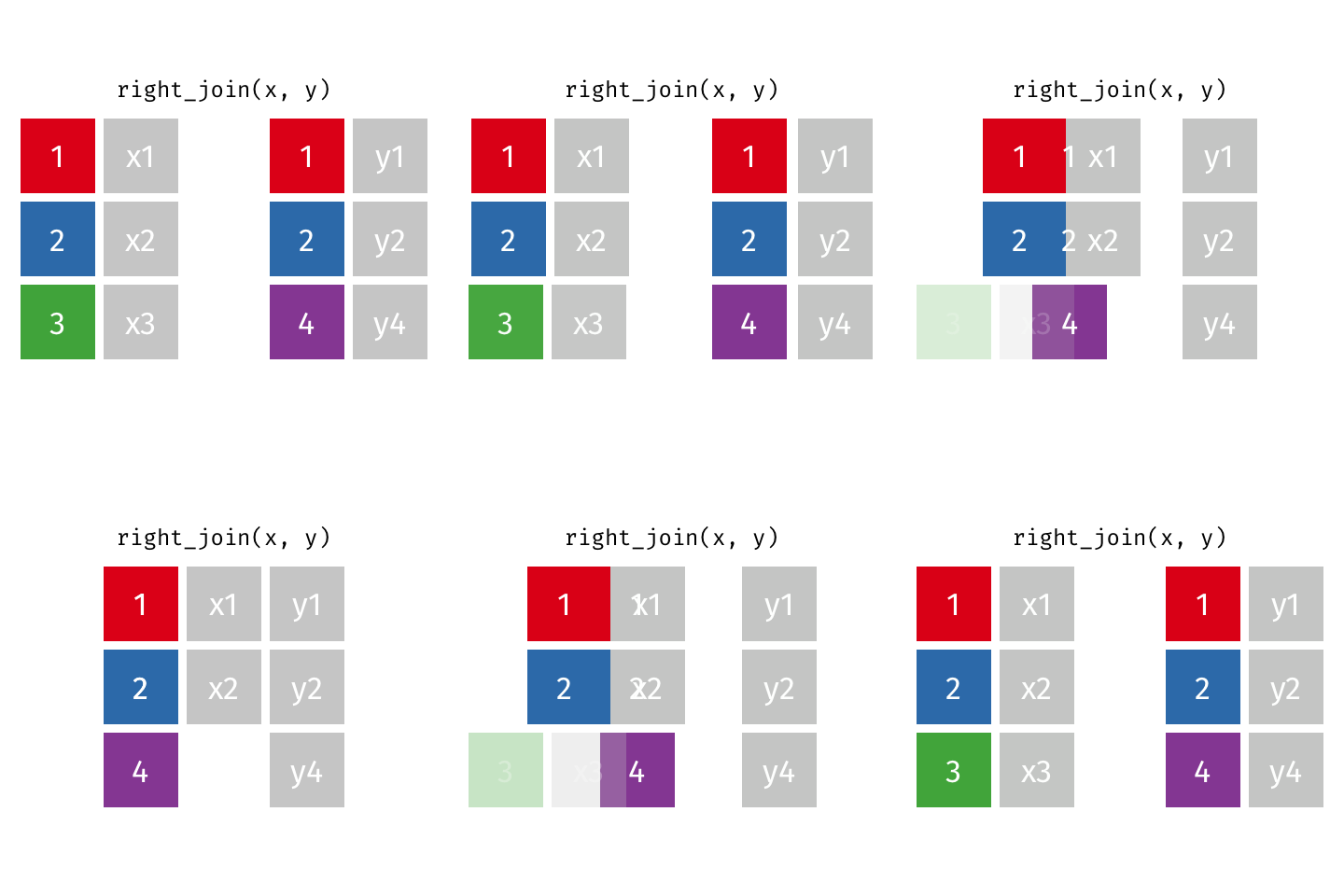
`right_join(df1, df2)`

Adds columns to df1 from df2, matching the cases in df2. Retains ALL cases from right data frame df2, and adds NA for variables from df1 that have no match.

df1

ID	name
1	x1
2	x2
3	x3

df2

ID	grade
1	y1
2	y2
4	y4

right_join(df1, df2, by = "ID")

ID	name	grade
1	x1	y1
2	x2	y2
4	NA	y4

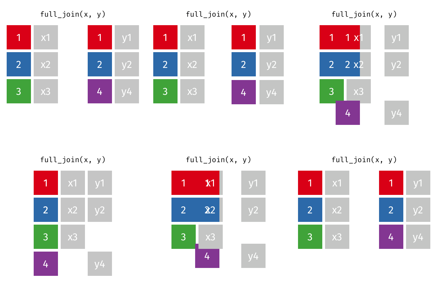
`full_join(df1, df2)`

Adds columns to df1 from df2, fully combining the two data frames, matching when possible. Retains ALL cases from df1 AND df2, and adds NAs as necesary.

df1

ID	name
1	x1
2	x2
3	x3

df2

ID	grade
1	y1
2	y2
4	y4

full_join(df1, df2, by = "ID")

ID	name	grade
1	x1	y1
2	x2	y2
3	x3	NA
4	NA	y4

`inner_join(df1, df2)`

Adds columns to df1 from df2, retaining only cases that exist in both df1 AND df2.

df1

ID	name
1	x1
2	x2
3	x3

df2

ID	grade
1	y1
2	y2
4	y4

inner_join(df1, df2, by = "ID")

ID	name	grade
1	x1	y1
2	x2	y2

Comprehension check

In which of the joins are NAs possibly introduced? In which of the joins are NAs never going to be introduced?
If we have some df1 and df2, in what scenario will the result of the four joins be the same? (i.e. what has to be true about df1 and df2?)
What do you think we call these “mutating” joins? Think about where we’ve seen that verb before!

Note: it’s possible to join on more than one variable!

Example

We have data on fishery harvests (in tons) by countries from 2016, stored in data frame fish:

fish |>
    slice(1:8)

country	capture	aquaculture
Afghanistan	1000	1200
Albania	7886	950
Algeria	95000	1361
American Samoa	3047	20
Andorra	0	0
Angola	486490	655
Antigua and Barbuda	3000	10
Argentina	755226	3673

Suppose I would like to explore the data on a continent level. We have another data frame called continent that looks like this:

continents |>
  slice(1:8)

Country	continent
Afghanistan	Asia
Åland Islands	Europe
Albania	Europe
Algeria	Africa
American Samoa	Oceania
Andorra	Europe
Angola	Africa
Anguilla	Americas

Discuss

fish data frame snapshot:

country	capture	aquaculture
Afghanistan	1000	1200
Albania	7886	950
Algeria	95000	1361
American Samoa	3047	20
Andorra	0	0

continents data frame snapshot:

Country	continent
Afghanistan	Asia
Åland Islands	Europe
Albania	Europe
Algeria	Africa
American Samoa	Oceania

We want to keep all rows and columns from fish and add a column for corresponding continents. Which join function should we use?
We want to keep only the rows from fish for which we have a corresponding continent and add a column for corresponding continents. Which join function should we use?
Which variable(s) are we joining on?

Example (cont.)

Question 1:

left_join(fish, continents, 
          by = c("country" = "Country")) |>
  slice(1:8)

country	capture	aquaculture	continent
Afghanistan	1000	1200	Asia
Albania	7886	950	Europe
Algeria	95000	1361	Africa
American Samoa	3047	20	Oceania
Andorra	0	0	Europe
Angola	486490	655	Africa
Antigua and Barbuda	3000	10	NA
Argentina	755226	3673	Americas

Notice the NA

Question 2:

inner_join(fish, continents, 
           by = c("country" = "Country")) |>
  slice(1:8)

country	capture	aquaculture	continent
Afghanistan	1000	1200	Asia
Albania	7886	950	Europe
Algeria	95000	1361	Africa
American Samoa	3047	20	Oceania
Andorra	0	0	Europe
Angola	486490	655	Africa
Argentina	755226	3673	Americas
Armenia	3758	16381	Asia

Notice we don’t have two copies of same country/Country variable!

Piping into `xxx_join()`

In the following line of code, when would an NA be introduced? (Answer forthcoming.)

right_join(fish, continents, by = c("country" = "Country"))

Remember in data wrangling, we pipe from a previous line of code directly into another
We can pipe directly into the join functions! The following achieves the same as above:

fish |>
  right_join(continents, by = c("country" = "Country"))

Answer to previous question

NAs would be introduced if there is a country in continents that does not appear in fish. See the last 50-ish cases:

Joins data frames and pivoting

Housekeeping

Pivoting

Wide data

Long data

Converting from wide -> long

pivot_longer()

Converting long -> wide

pivot_wider()

pivot_wider()

Joins

Joining data frames

Setup

left_join(df1, df2)

right_join(df1, df2)

full_join(df1, df2)

inner_join(df1, df2)

Comprehension check

Example

Discuss

Example (cont.)

Piping into xxx_join()

Answer to previous question

`left_join(df1, df2)`

`right_join(df1, df2)`

`full_join(df1, df2)`

`inner_join(df1, df2)`

Piping into `xxx_join()`