Simpson’s paradox

2025-10-02

Study design recap

• What are the differences between observational studies and experimental studies?

• What is a confounding variable?

UC Berkeley admissions

Observational study on sex bias based on Fall 1973 admissions data to the graduate program at the University of California, Berkeley

	Admit	Deny	Total
Men	3738	4704	8442
Women	1494	2827	4321
Total	5232	7531	12763

1. What is the probability* of admission for a randomly selected applicant?

2. What is the probability of admission among men? Among women?

3. Are the probabilities you found marginal, joint, or conditional probabilities?

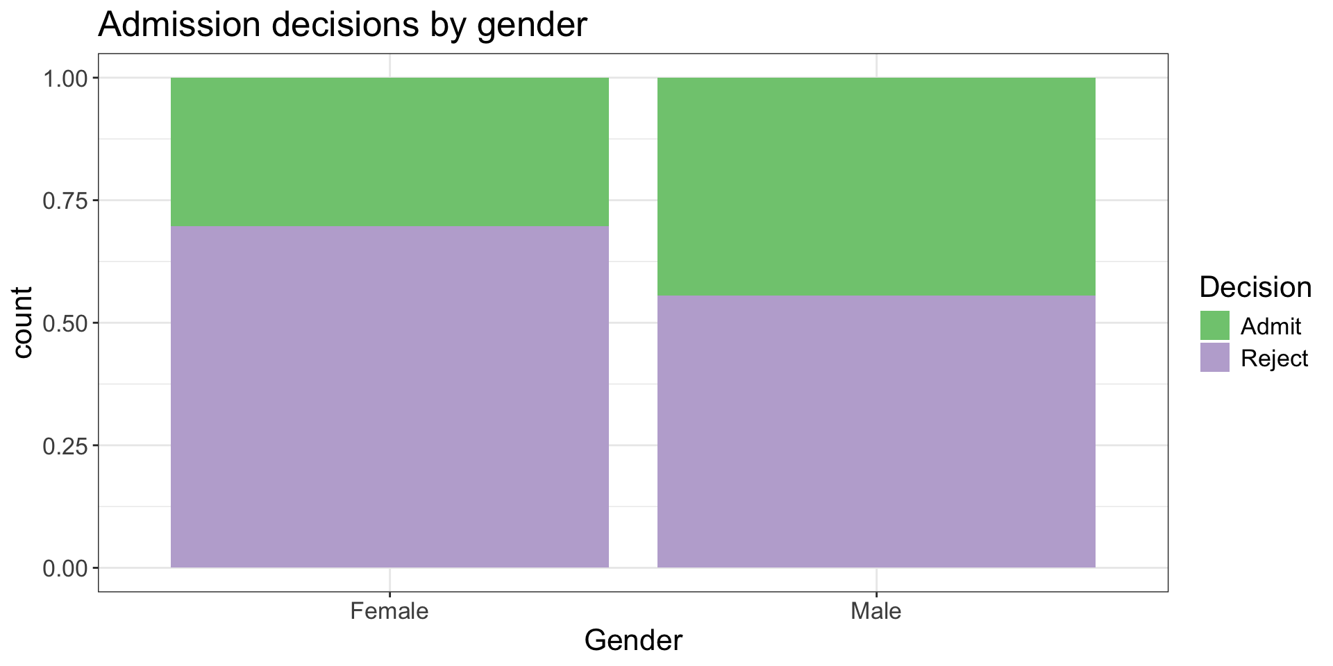
Suppose we want to understand the relationship between gender and admission decision. What sort of visualization might be appropriate for representing this data?

UC Berkeley admissions (cont.)

Case study

An application of probability!

Dive into data

We have more nuanced data about the graduate admissions: we know the department that each person was applied to.

We will consider the six largest departments: A, B, C, D, E, F

• The first six observations in the data frame are as follows:

# head() gives us the first 6 rows
head(admissions)

# A tibble: 6 × 3
  Decision Gender Dept 
  <chr>    <chr>  <chr>
1 Admit    Male   B    
2 Reject   Female C    
3 Admit    Male   C    
4 Reject   Female C    
5 Admit    Male   A    
6 Reject   Male   F    

• What sort of EDA would be interesting/appropriate for these data?

Frequency tables

Number of applicants by department:

Female applicants:

admissions |>
  filter(Gender == "Female") |> 
  count(Dept)

Dept	n
A	108
B	25
C	593
D	375
E	393
F	341

Male applicants:

admissions |>
  filter(Gender == "Male") |> 
  count(Dept)

Dept	n
A	825
B	560
C	325
D	417
E	191
F	373

Both groups:

admissions |>
  count(Dept, Gender)

Dept	Gender	n
A	Female	108
A	Male	825
B	Female	25
B	Male	560
C	Female	593
C	Male	325
D	Female	375
D	Male	417
E	Female	393
E	Male	191
F	Female	341
F	Male	373

More-detailed frequency tables

Number of applicants by department and admission status:

Female applicants:

Dept	Decision	n
A	Admit	89
A	Reject	19
B	Admit	17
B	Reject	8
C	Admit	202
C	Reject	391
D	Admit	131
D	Reject	244
E	Admit	94
E	Reject	299
F	Admit	24
F	Reject	317

Male applicants:

Dept	Decision	n
A	Admit	512
A	Reject	313
B	Admit	353
B	Reject	207
C	Admit	120
C	Reject	205
D	Admit	138
D	Reject	279
E	Admit	53
E	Reject	138
F	Admit	22
F	Reject	351

Visualize

Can visualize three categorical variables at once!

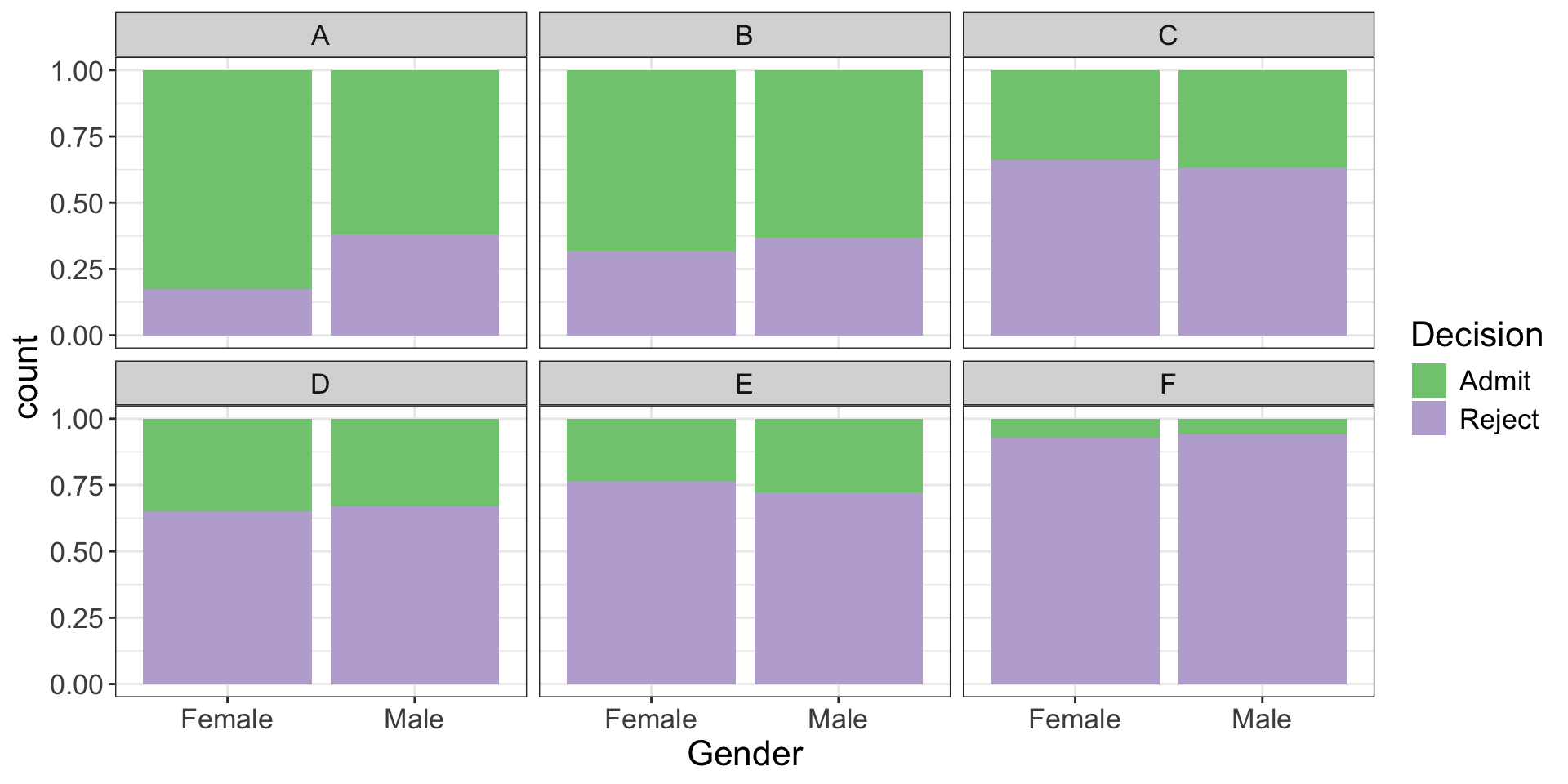
Closer look

Probability of admission conditioning on gender and department:

Dept	Gender	cond_prob_admit
A	Female	0.82
A	Male	0.62
B	Female	0.68
B	Male	0.63
C	Female	0.34
C	Male	0.37
D	Female	0.35
D	Male	0.33
E	Female	0.24
E	Male	0.28
F	Female	0.07
F	Male	0.06

• Are all departments uniform in admission rates?
• Do admissions still seem biased against female applicants?

What’s going on?

• But wait… didn’t we start by noting that men were way more likely to be admitted than women?

• The first two departments (A and B) are easy to get into

• The following table shows for each gender, the proportion of applicants each department received.

Gender	Dept	cond_prop
Female	A	0.059
Female	B	0.014
Female	C	0.323
Female	D	0.204
Female	E	0.214
Female	F	0.186
Male	A	0.307
Male	B	0.208
Male	C	0.121
Male	D	0.155
Male	E	0.071
Male	F	0.139

What do you notice?

Simpson’s paradox

The UC Berkeley admissions observational study is an example of Simpson’s paradox: when omitting one explanatory variable causes the measure/degree of association between another explanatory variable and a response variable to reverse or disappear

• In other words, the inclusion/exclusion of a third variable in the analysis can change the apparent relationship between the other two variables

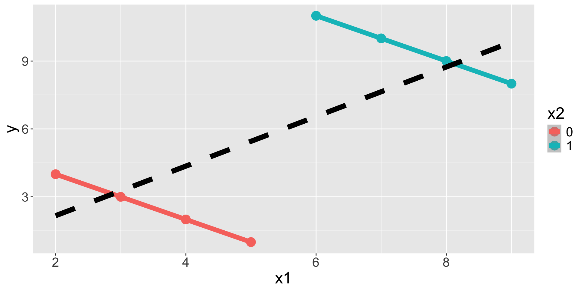
• What was the confounding variable in UC Berkeley study?

Live code

• Using wrangling to obtain probabilities

• case_when() to create more complex categorical variables

Wrangling for probabilities

What is the probability that someone was admitted?

admissions |>
  count(Decision) |>
  mutate(prob = n/sum(n)) |>
  select(-n)

# A tibble: 2 × 2
  Decision  prob
  <chr>    <dbl>
1 Admit    0.388
2 Reject   0.612

What is the probability that someone was admitted, conditioned on gender?

admissions |>
  count(Gender, Decision) |>
  group_by(Gender) |>
  mutate(cond_prob = n/sum(n)) |>
  select(-n)

# A tibble: 4 × 3
# Groups:   Gender [2]
  Gender Decision cond_prob
  <chr>  <chr>        <dbl>
1 Female Admit        0.304
2 Female Reject       0.696
3 Male   Admit        0.445
4 Male   Reject       0.555

• How might I extend to also condition on Department?

More complex categorical variables

Suppose I want to create a new variable called Dept2 that takes the values:

• “Group 1” if someone applied to Department A or B
• “Group 2” if someone applied to Department C or D
• “Group 3” if someone applied to Department E or F

# option 1 (awful): nested if_else()
admissions |>
  mutate(Dept2 = if_else(Dept %in% c("A", "B"), "Group 1",
                           if_else(Dept %in% c("C", "D"), "Group 2",
                                   "Group 3")))

# A tibble: 5 × 4
  Decision Gender Dept  Dept2  
  <chr>    <chr>  <chr> <chr>  
1 Reject   Female C     Group 2
2 Admit    Male   A     Group 1
3 Reject   Female E     Group 3
4 Reject   Male   B     Group 1
5 Reject   Female C     Group 2

case_when()

We will use the case_when() function which generalizes if_else(). We use the following notation: <logical condition> ~ <value of variable>. Different “ifs” are separated by commas, and the logical conditions are checked sequentially.

admissions |>
  mutate(Dept2 = case_when(
    Dept %in% c("A", "B") ~ "Group 1",
    Dept %in% c("C", "D") ~ "Group 2",
    Dept %in% c("E", "F") ~ "Group 3",
  )) 

# A tibble: 5 × 4
  Decision Gender Dept  Dept2  
  <chr>    <chr>  <chr> <chr>  
1 Reject   Female C     Group 2
2 Admit    Male   A     Group 1
3 Reject   Female E     Group 3
4 Reject   Male   B     Group 1
5 Reject   Female C     Group 2

# The following is also acceptable, but 
# relies on sequential ordering:
admissions |>
  mutate(Dept2 = case_when(
    Dept %in% c("A", "B") ~ "Group 1",
    Dept %in% c("C", "D") ~ "Group 2",
    T ~ "Group 3",
  )) |>
  sample_frac() 

# A tibble: 5 × 4
  Decision Gender Dept  Dept2  
  <chr>    <chr>  <chr> <chr>  
1 Reject   Female C     Group 2
2 Admit    Male   A     Group 1
3 Reject   Female E     Group 3
4 Reject   Male   B     Group 1
5 Reject   Female C     Group 2

Prettier tables using kable()

• When we finish wrangling, the output is always a data frame

  • While this is so useful for coding, it’s not the most beautiful when rendering!

  • How can we make turn the data frame into a beautiful table?

• We will need to first install the kableExtra library.

Currently:

admissions |>
  count(Decision) |>
  mutate(prob = n/sum(n))

# A tibble: 2 × 3
  Decision     n  prob
  <chr>    <int> <dbl>
1 Admit     1755 0.388
2 Reject    2771 0.612

• Using kable() (note we can specify number of digits)

library(kableExtra)
admissions |>
  count(Decision) |>
  mutate(prob = n/sum(n)) |>
  kable(digits = 3) 

Decision	n	prob
Admit	1755	0.388
Reject	2771	0.612