Bootstrap Confidence Intervals
2025-10-15
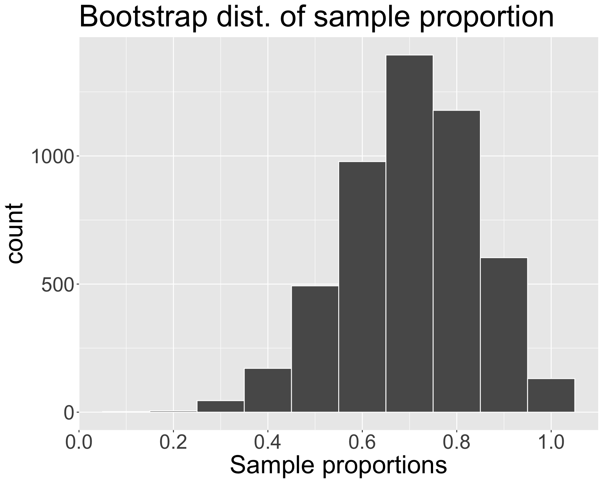
Bootstrap distribution from activity
In our original sample of \(n = 10\), we had \(\widehat{p_{obs}} = 0.7\).
We have the following bootstrap distribution of sample proportions, obtained from \(B=\) 5000 iterations:
We can compare to the true sampling distribution (because it’s easy for me to re-sample from the population here):
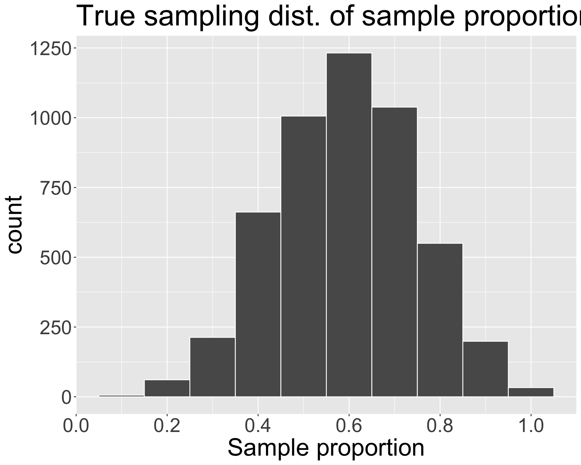
- Notice that our bootstrap distribution isn’t a great approximation (maybe \(n = 10\) did not yield a representative sample)
Visualizing bootstrap confidence interval
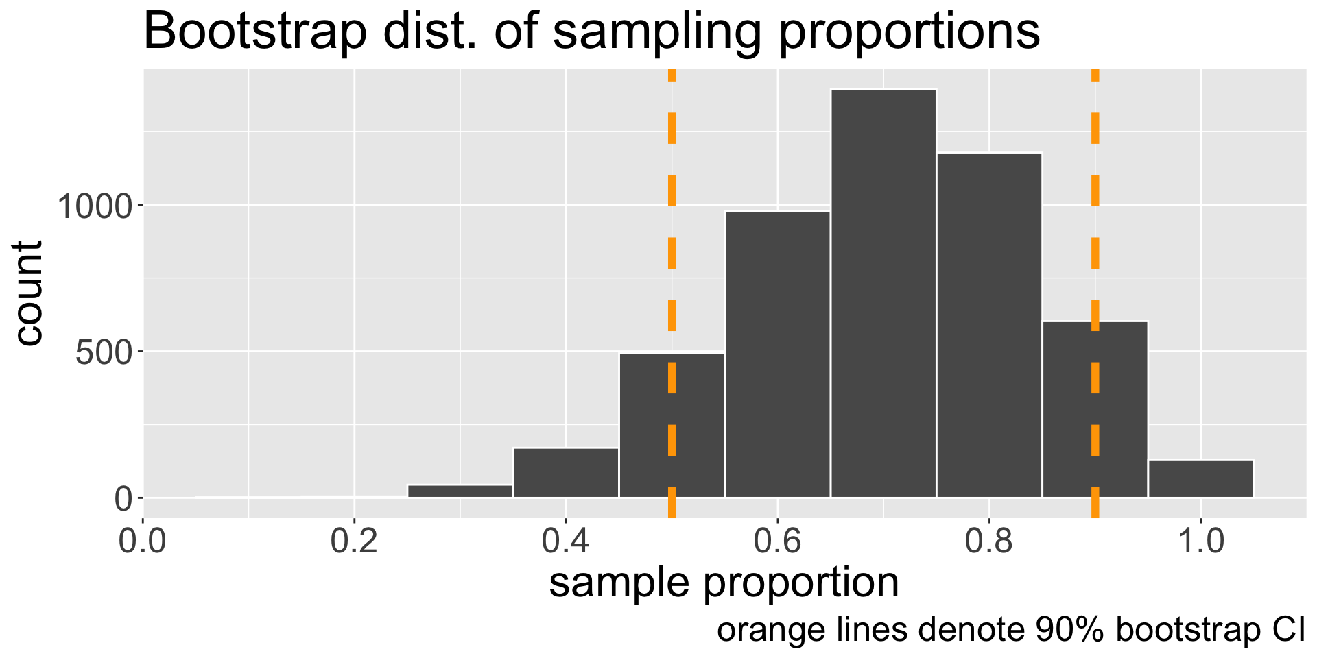
- Our 90% bootstrap CI for \(p\): (0.5, 0.9)
Comparing confidence intervals
Comparing changes in 90% bootstrap CI for sample sizes \(n = 5, 10, \text{ and } 20\).
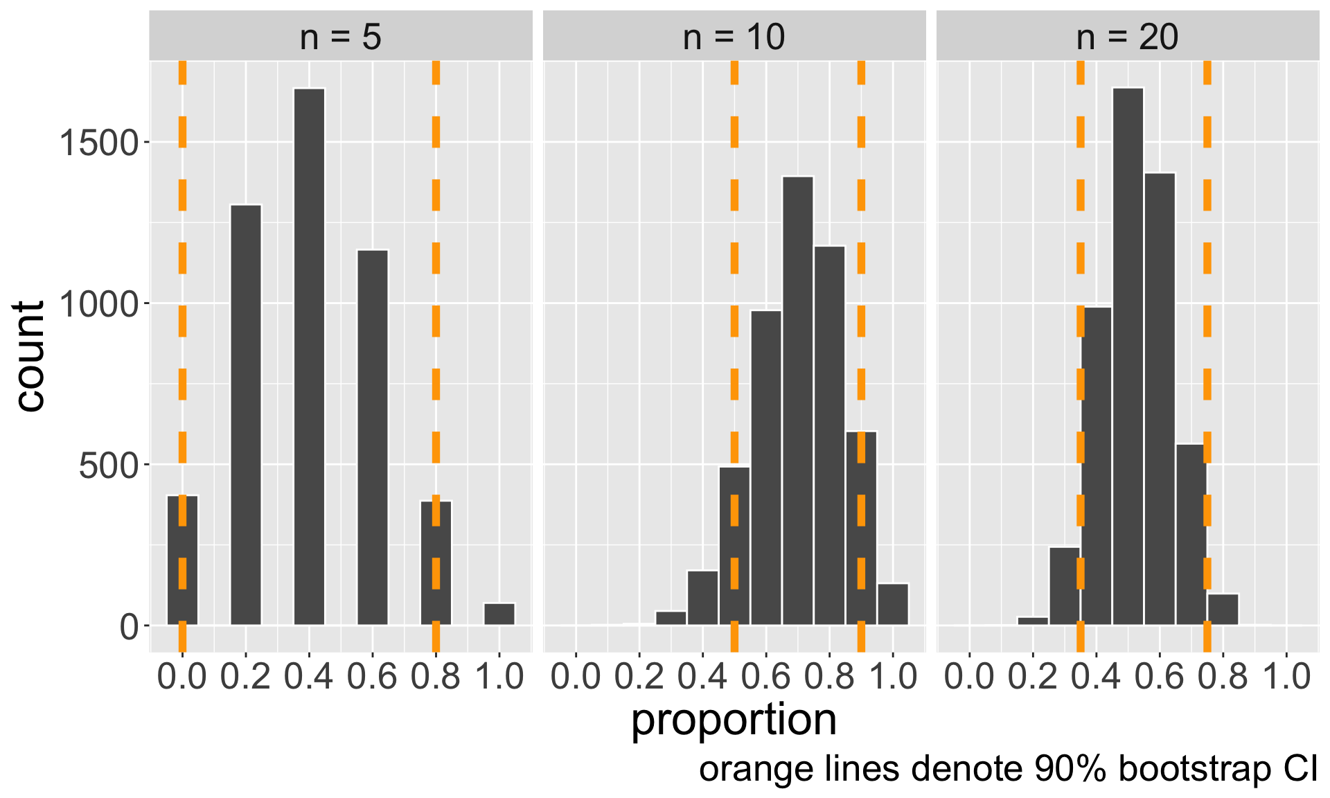
| n | interval |
|---|---|
| n = 5 | (0, 0.8) |
| n = 10 | (0.5, 0.9) |
| n = 20 | (0.35, 0.75) |
What do you notice about the bootstrap distributions and CIs as \(n\) increases?
In-line code
In-line code allows us to be reproducible! Suppose I do all this analysis:
[1] 0.7I might want to report this value! Rather than “hard-code” the value 0.7 in the white text of my .qmd, I want the .qmd to update the value dynamically upon rendering!
.qmd file 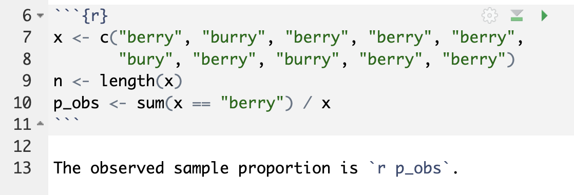
Rendered PDF 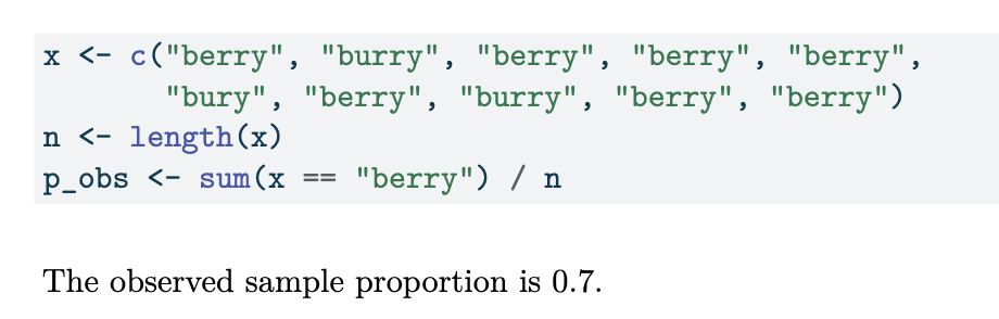
- Notice the syntax of inline code! Backticks, r, and the spacing matter!