| sex | not promote | promote | total |
|---|---|---|---|
| female | 10 | 14 | 24 |
| male | 3 | 21 | 24 |
| total | 13 | 35 | 48 |
Hypothesis Testing via Randomization
2025-10-20
Where we’re going today
We will see another kinds of hypotheses for different types of research questions
Hypothesis testing framework is the same, but will change how we obtain null distribution
Try to see the big picture
Test of independence
Running example: sex discrimination study
Note: this study considered sex as binary “male” or “female”, and did not take into consideration gender identities
Participants in the study were 48 bank supervisors who identified as male and were attending a management institute at UNC in 1972
Each supervisor was asked to assume the role of personnel director of a bank
Each given a file to judge whether the person in the file should be promoted
The files were identical, except half of them indicated that the candidate was male, and the other half were indicated as female
Files were randomly assigned to bank managers
Experiment or observational study?
Research question: Are individuals who identify their sex as female discriminated against in promotion decisions made by their managers who identify as male?
Defining hypotheses
Research question: Are individuals who identify their sex as female discriminated against in promotion decisions made by their managers who identify as male?
What is/are the variables(s) here? What types of variables are they?
We need to construct hypotheses where \(H_{0}\) is “status quo” and \(H_{A}\) is the claim researchers have
\(H_{0}\): the variables
sexanddecisionare independent.- i.e. any observed difference in promotion rates is due to variability
\(H_{A}\): the variables
sexanddecisionare not independent; equally-qualified female personnel are less likely to be promoted than male personnel
Data
For each of the 48 supervisors, the following were recorded:
The sex of the candidate in the file (male/female)
The decision (promote/not promote)
- What evidence do we have? What summary statistic(s) would be useful for answering the research question?
Data (cont.)
Conditional probability of getting promoted by sex:
| sex | decision | cond_prob |
|---|---|---|
| female | promote | 0.583 |
| male | promote | 0.875 |
Is the observed difference \(\hat{p}_{f,obs} - \hat{p}_{m,obs} =\) -0.2916667 convincing evidence? We need to examine variability in the data, assuming \(H_{0}\) true.
Let’s set \(\alpha = 0.05\)
Simulate under null
Simulating under \(H_{0}\) means operating in a hypothetical word where
sexanddecisionare independent.- This means that knowing the
sexof the candidate should have no bearing on thedecisionto promote or not
- This means that knowing the
We will perform a simulation called a randomization test:
Randomly pair up
decisionandsexoutcome pairsRandomly assigning a decision to each person would be equivalent to a world in which the bankers’
decisionhad been independent of candidate’ssex(i.e. if \(H_{0}\) true)
Randomization test
| sex | not promote | promote | total |
|---|---|---|---|
| female | 10 | 14 | 24 |
| male | 3 | 21 | 24 |
| total | 13 | 35 | 48 |
Write down “promote” on 35 cards and “not promote” on 13 cards. Repeat the following:
Thoroughly shuffle these 48 cards.
Deal out a stack of 24 cards to represent males, and the remaining 24 cards to represent females
- This is how we simulate under \(H_{0}\)
Calculate the proportion of “promote” cards in each stack, \(\hat{p}_{f, sim}\) and \(\hat{p}_{m, sim}\)
Calculate and record the difference \(\hat{p}_{f,sim} - \hat{p}_{m,sim}\) (order of difference doesn’t matter so long as you are consistent)
Randomization test (activity)
Try it!
Randomization test (code)
set.seed(100)
n <- nrow(discrimination)
n_f <- sum(discrimination$sex == "female")
n_m <- sum(discrimination$sex == "male")
decisions <- discrimination$decision
B <- 1000
diff_props_null <- rep(NA, B)
for(b in 1:B){
  shuffled <- sample(decisions, n)
  rand_f <- shuffled[1:n_f]
  rand_m <- shuffled[-c(1:n_f)]

  p_f_sim <-  mean(rand_f == "promote")
  p_m_sim <-mean(rand_m == "promote")

  diff_props_null[b] <- p_f_sim - p_m_sim
}- Where should the null distribution be centered?
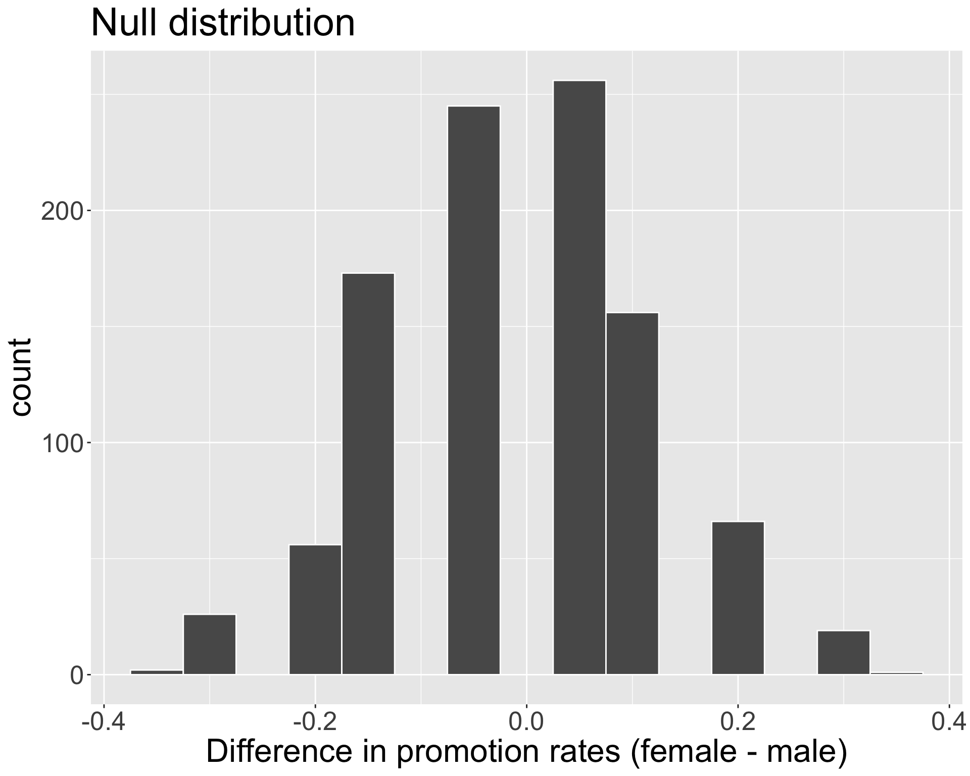
Null distribution
Obtain p-value
Recall, the observed difference in our data was \(\hat{p}_{f,obs} - \hat{p}_{m,obs} =\) -0.2916667.
p-value is probability of observing data as or more extreme than our original data, given \(H_{0}\) true.
Where does “as or more extreme” correspond to on our plot?
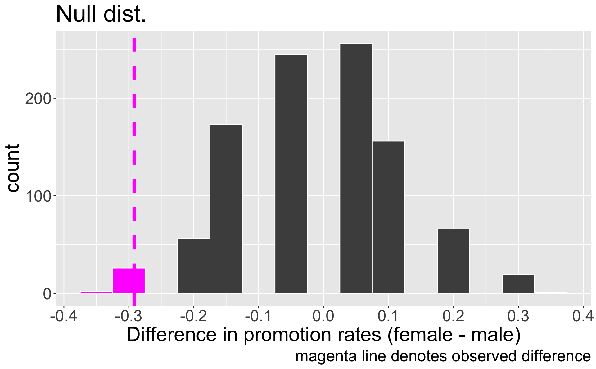
- Out of 1000 simulations under \(H_{0}\), 28 resulted in a difference in promotion rates as or more extreme than our observed
- So the p-value is approximately 0.028
Making decision and conclusion
Our research question: Are individuals who identify their sex as female discriminated against in promotion decisions made by their managers who identify as male?
- \(H_{0}\):
sexanddecisionare independent - \(H_{A}\):
sexanddecisionare not independent and equally-qualified female personnel are less likely to get promoted than male personnel by male supervisors - \(\alpha = 0.05\)
Interpret our p-value in context.
Make a decision and conclusion in response to the research question.
Making decision and conclusion (answer)
p-value interpretation: Assuming that
sexanddecisionare independent, the probability of observing a difference in promotion rates as or more extreme as -0.2916667 is 0.028.Decision: Because the observed p-value of 0.028 is less than our significant level 0.05, we reject \(H_{0}\).
Conclusion: The data provide strong evidence of sex discrimination against female candidates by the male supervisors.
What kind of error could we have made?
Difference in two proportions
Running example: CPR
An experiment was conducted, consisting of two treatments on 90 patients who underwent CPR for a heart attack and subsequently went to the hospital. Each patient was randomly assigned to either:
- treatment group: received a blood thinner
- control group: did not receive a blood thinner
For each patient, the outcome recorded was whether they survived for at least 24 hours.
What is/are the variables(s) here? What types of variables are they?
Defining hypotheses
Research question: For patients who undergo CPR after a heart attack, does the blood thinner treatment have an effect on survival?
\(H_{0}:\) the blood thinner treatment has no effect on survival after heart attack
\(H_{A}:\) the blood thinner treatment has an effect on survival after heart attack
Try to write down the hypotheses using statistical notation.
- Let \(p_{T}\) and \(p_{C}\) denote the proportion of patients who survive when receiving the thinner (Treatment) and when not receiving the treatment (Control), respectively
Option 1
\(H_{0}\): \(p_{T} = p_{C}\)
\(H_{A}\): \(p_{T} \neq p_{C}\)
Option 2 (preferred)
\(H_{0}\): \(p_{T} - p_{C} = 0\)
\(H_{A}\): \(p_{T} - p_{C} \neq 0\)
Collect data
Using the data, obtain the observed difference in sample proportions.
# A tibble: 3 × 2
  group     outcome
  <fct>     <fct>
1 treatment died
2 control   died
3 control survived| group | died | survived | total |
|---|---|---|---|
| control | 39 | 11 | 50 |
| treatment | 26 | 14 | 40 |
| total | 65 | 25 | 90 |
- What evidence do we have? What summary statistic(s) would be useful for answering the research question?
Summarise data
| group | died | survived | total |
|---|---|---|---|
| control | 39 | 11 | 50 |
| treatment | 26 | 14 | 40 |
| total | 65 | 25 | 90 |
\(\hat{p}_{C, obs} = \frac{11}{50} = 0.22\)
\(\hat{p}_{T,obs} = \frac{14}{40} = 0.35\)
Observed difference: \(\hat{p}_{T,obs} - \hat{p}_{C,obs} = 0.13\)
Is this “convincing evidence” that blood thinner usage after CPR has an effect on survival?
Set \(\alpha = 0.05\)
Simulate under null
We will once again perform a randomization test to try and simulate the difference in proportions under \(H_{0}\)
- Under \(H_{0}\), treatment group is no better than control group, so let’s simulate assuming that outcome and treatment are independent
- Try filling out worksheet!
Write down
diedon 65 cards, andsurvivedon 25 cards. Then repeat several times:Shuffle cards well
Deal out 50 to be Control group, and remaining 40 to be Treatment group
Calculate proportions of survival \(\hat{p}_{C, sim}\) and \(\hat{p}_{T, sim}\)
Obtain and record the simulated difference \(\hat{p}_{T, sim} - \hat{p}_{C, sim}\)
Simulate under null (code)
Live code or look here:
set.seed(310)
n_t <- sum(cpr$group == "treatment")
n_c <- sum(cpr$group == "control")
cards <- cpr$outcome
B <- 1000
diff_props_null <- rep(NA , B)
for(b in 1:B){
  shuffled <- sample(cards)
  treat_sim <- shuffled[1:n_t]
  control_sim <- shuffled[-c(1:n_t)]

  p_t_sim <- mean(treat_sim == "survived")
  p_c_sim <- mean(control_sim == "survived")

  diff_props_null[b] <- p_t_sim - p_c_sim
}
Where should our null distribution be centered at?
Visualizing null distribution
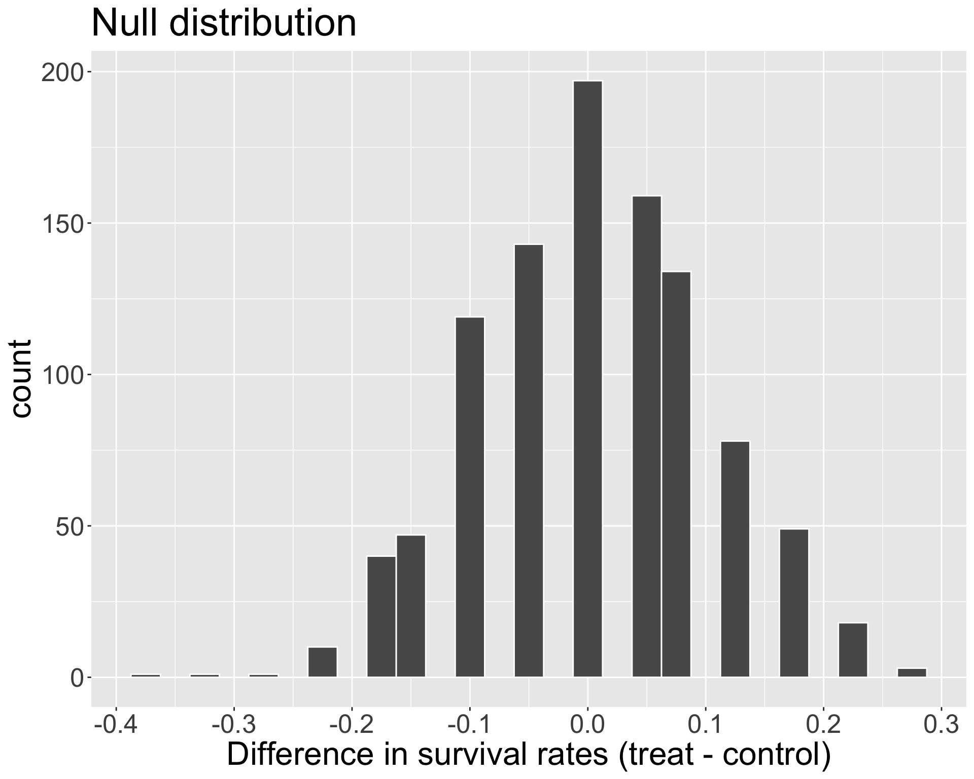
How would we obtain the p-value in this problem? What does it mean to be “as or more extreme” in the direction of \(H_{A}\)?
Calculate p-value
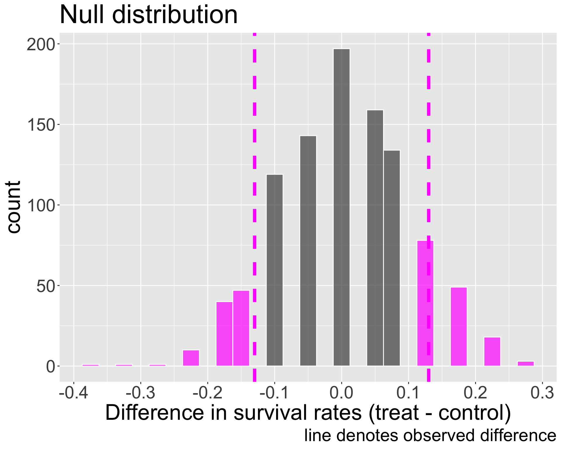
We simulated 248 out of 1000 simulations where the difference in proportions under \(H_{0}\) was as or more extreme than our observed difference of 0.13
So p-value is approximately 0.248
Interpret and make conclusion
The researchers are interested in learning if the blood thinner treatment has an effect on survival after heart attack.
Our p-value is 0.248.
- Make a decision and conclusion about the research question in context. What type of error could we have made?
Decision: because our p-value of 0.248 is greater than \(\alpha = 0.05\), we fail to reject \(H_{0}\)
Conclusion: the data do not provide convincing evidence that the blood thinner treatment affects survival rates among patients who undergo CPR.
Possible error: Type 2
Comprehension questions
What were the similarities and differences between:
hypothesis test for independence
hypothesis test for two proportions
How do the randomization tests today differ from the test for one proportion that we learned last class?