Hypothesis testing for a mean

2025-10-23

Housekeeping

• Make sure to start working on Problem Set 6!

Recap

• We have seen how to perform hypothesis tests for questions involving the following:

  • A single proportion (Middle “berry” vs “burry”)

  • Independence of two categorical variables (banker sex discrimination)

    • Think of as one population

  • Difference in two proportions (blood thinner)

    • Think of as two populations

• We are now going to see another hypothesis test, this time for numerical data

Test for a single mean

Running example + form hypotheses

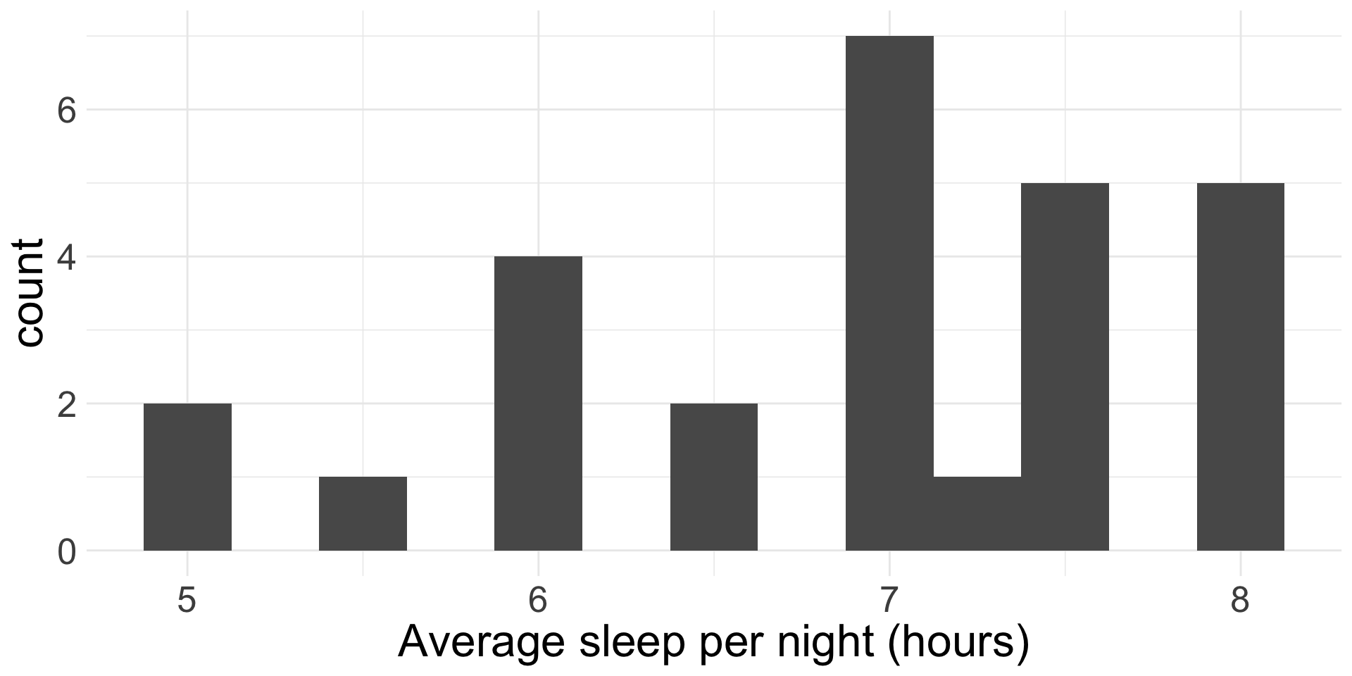
We will use the the data I collected from you about average hours of sleep per night.

What type of variable(s) do we have?

• I know most college students don’t receive the recommended 8 hours of sleep. But what about 7.5 hours?

• Before we look at the data, we should form our hypotheses. Suppose I am interested in learning if Middlebury students who have an 8:15am class get at most 7.5 hours of sleep (on average).

• What might our hypotheses be?

  • \(H_{0}\): \(\mu =\) 7.5 versus \(H_{A}\): \(\mu <\) 7.5, where \(\mu\) is the true mean of the average hours of sleep Middlebury students with an 8:15 am class get.
    • Terminology: I will refer to \(\mu_{0} =\) 7.5 as my “null hypothesized value”. (i.e. the specific value of \(\mu\) in \(H_{0}\))

Collect and summarise data

The observed/sample mean of average hours of sleep per night is \(\bar{x}_{obs} =\) 6.896 from a sample of 27 students

• Now we must determine if we have “convincing evidence”! Choose \(\alpha = 0.05\)

Simulating null distribution

To simulate from the null distribution, we need to operate in a world where \(H_{0}\) is true.

• So, I need to repeatedly simulate data sets of size 27 where true mean is \(\mu_{0} =\) 7.5, without changing anything else

  • Specifically, my hypotheses aren’t saying anything about spread, just center!

• If I don’t want to make any assumptions about how the data behave, how might I do that?

Recap bootstrap (NOT exactly the strategy)

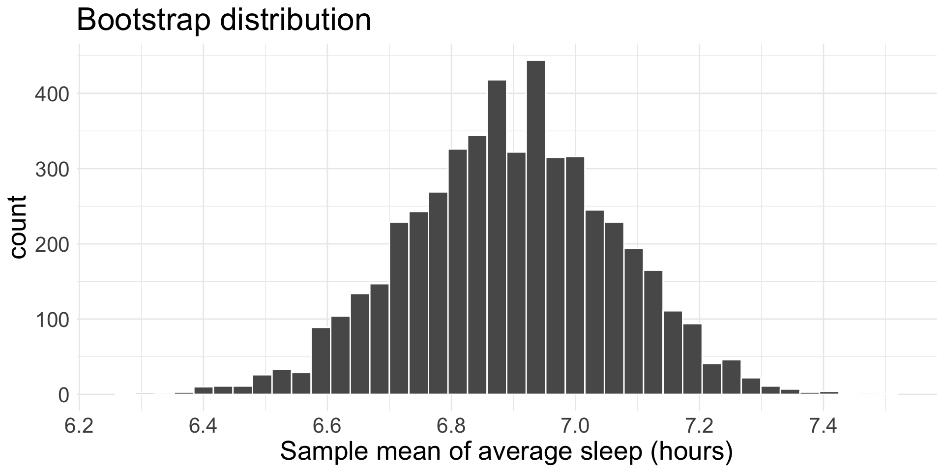
How would I obtain a bootstrap distribution of the sample mean of mean hours of sleep?

Remind ourselves: Where should the bootstrap distribution be centered?

Bootstrap to null distribution

• This is not the null distribution! The null distribution should be centered at \(\mu_{0} = 7.5\)

• However, the null distribution should have the same variability in \(\bar{x}\) as the bootstrap distribution.

• So to get the null distribution, why not just shift the bootstrap distribution to be centered where we want it to be?

Shifting the bootstrap distribution

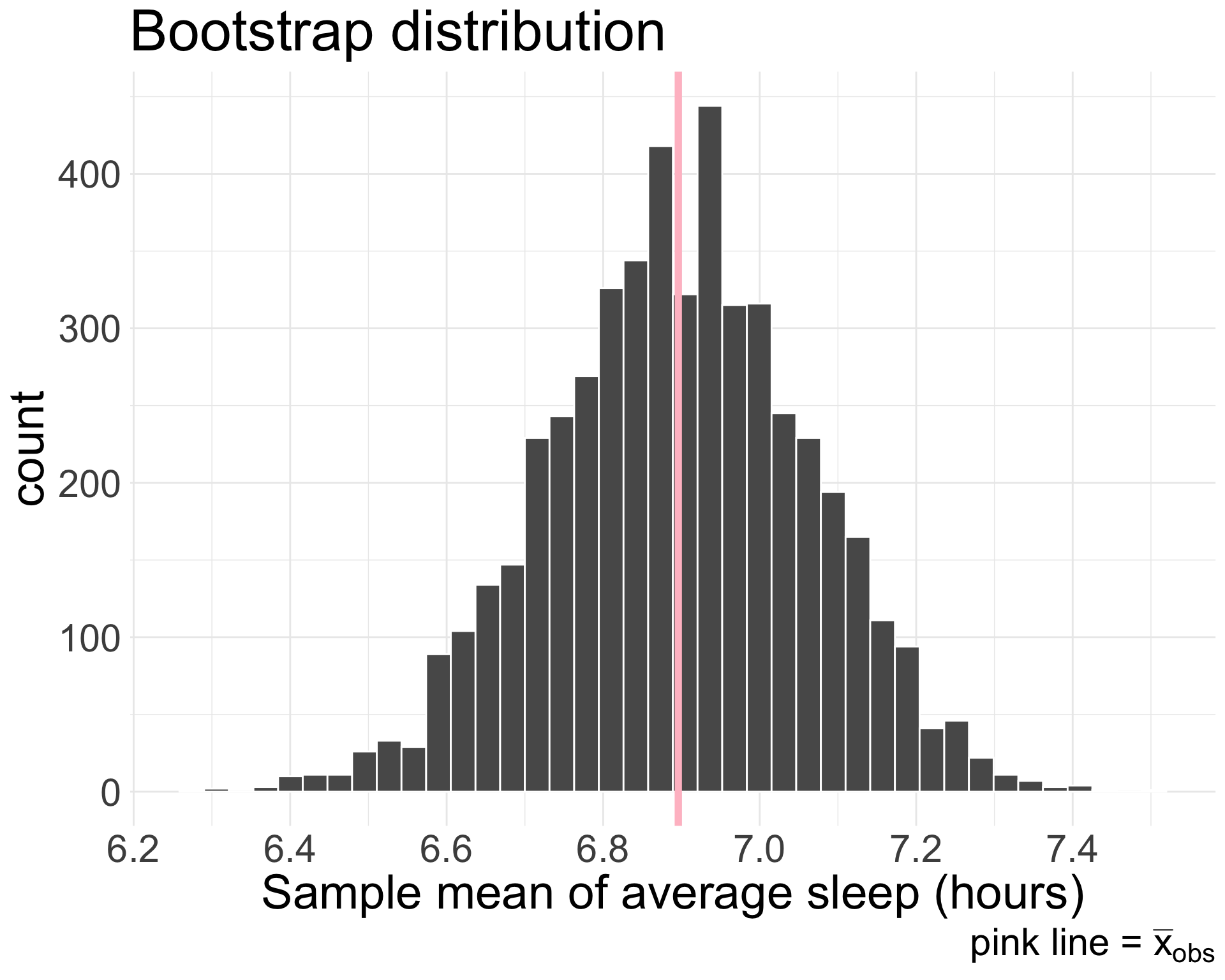
• In this example, bootstrap distribution is centered at \(\bar{x}_{obs} = 6.896\)

• In order to center this distribution at \(\mu_{0} = 7.5\), just subtract \(6.896 - 7.5 = -0.604\) from every single bootstrapped mean

  • This will give us a simulated distribution for \(\bar{x}\) centered at \(\mu_{0} = 7.5\), which is exactly the null distribution!

  • We call this “shifting the bootstrap distribution”, because we simply shift where the bootstrap distribution is centered

mu0 <- 7.5

# xbar holds observed sample mean
shift <- xbar - mu0

# boot_means is a vector holding B bootstrapped sample means
null_dist <- boot_means - shift

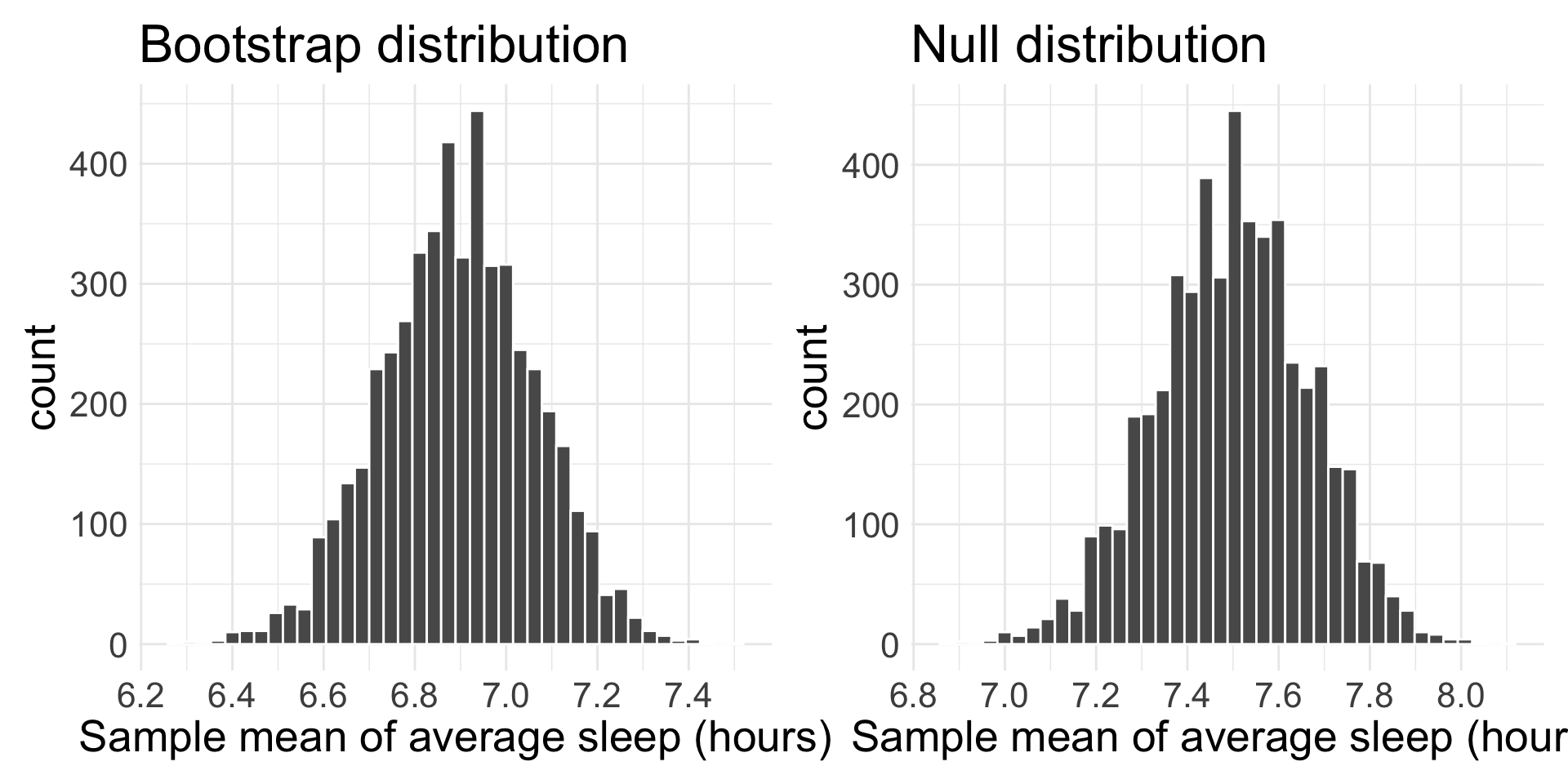
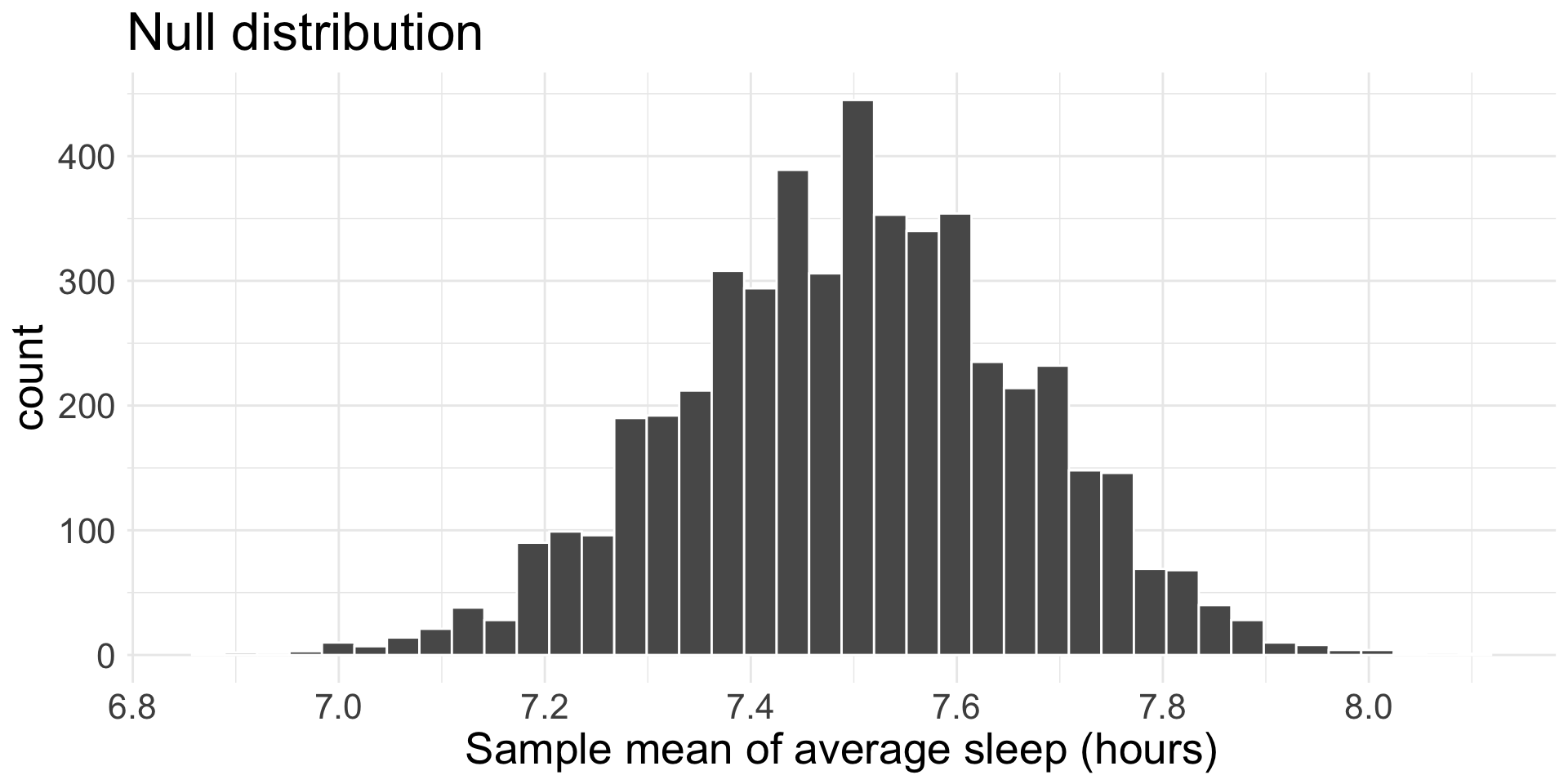
Null distribution

• Notice where the distributions are centered. Also note: graphs aren’t exactly identical due to binning of histogram.

Obtain the p-value

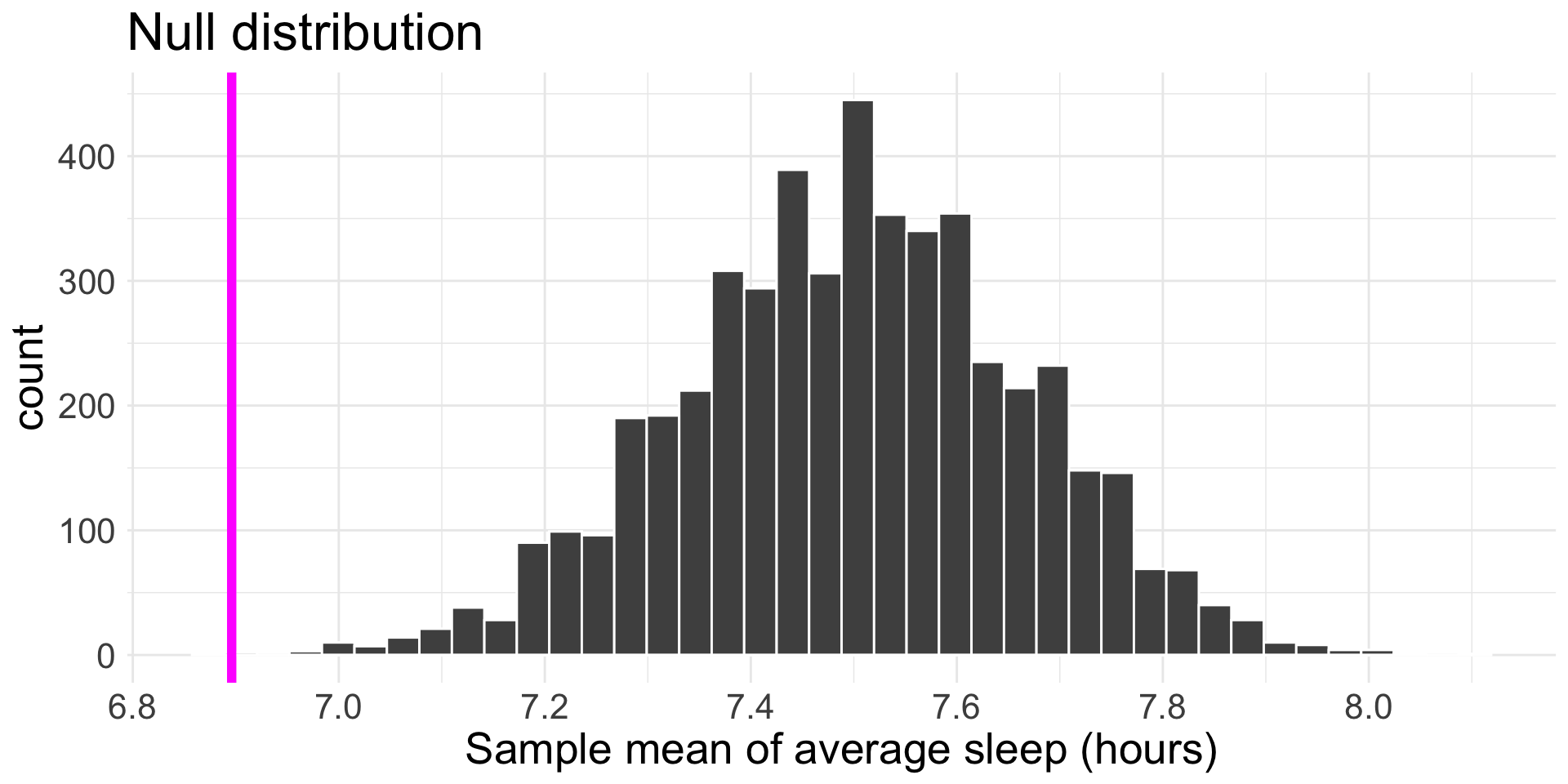
\(H_{0}\): \(\mu =\) 7.5 versus \(H_{A}\): \(\mu <\) 7.5

Our observed sample mean is \(\bar{x}_{obs} =\) 6.896.

How do we find our p-value?

• In 5000 iterations, simulated 1 “as more extreme” than our data, so p-value is approximately 0.0002.

Make decision and conclusion

Make a decision and conclusion in the context of the research question.

• Since our p-value of 0.0002 is less than the significance level of 0.05, we reject \(H_{0}\). We have convincing evidence to suggest that the true mean of the average hours of sleep per night that a Middlebury student with an 8:15am course receives per night is less than 7.5 hours.

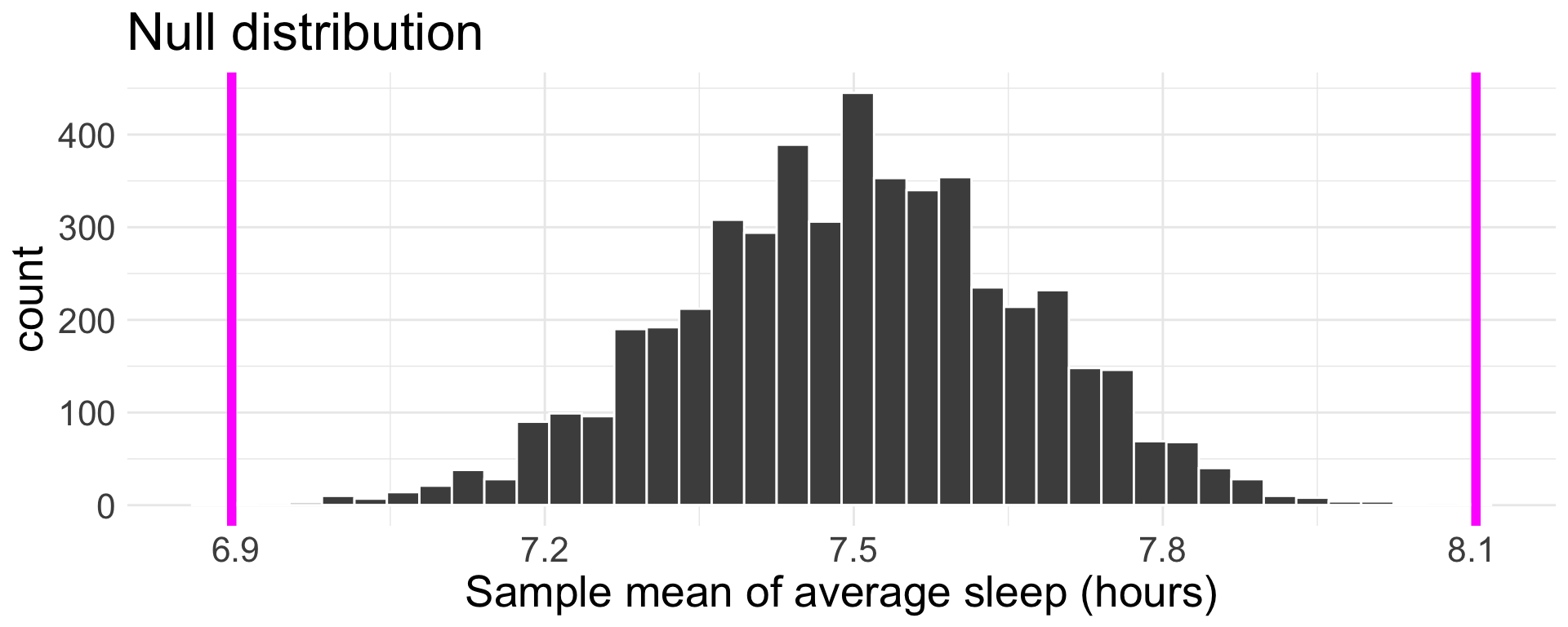
Two-sided alternative hypothesis

What if instead, I am interested in learning if Middlebury students who have an 8:15am class get 7.5 hours of sleep or not (on average). Then our hypotheses are:

\[H_{0}: \mu = 7.5 \qquad \text{ vs. } \qquad H_{A}: \mu \neq 7.5\]

• What does it mean to be “as or more extreme” now? Remember, \(\bar{x}_{obs} = 6.896\)

Two-sided alternative hypothesis

We can be extreme in both the positive and negative direction of \(\mu_{0}\)!

• Note that there are now 2 simulations that are “as or more extreme”, so p-value is approximately 0.0004.

Obtain the p-value (cont.)

Let \(shift\) represent the amount we shifted the bootstrap distribution by:

\[shift = 6.896 - 7.5 = -0.604\]

• Simulated sample means as or more extreme as the following will contribute:

  • \(\mu_{0} + shift = 7.5 + -0.604 = 6.896\) , or

  • \(\mu_{0} - shift = 7.5 - -0.604 = 8.104\)

• Note that how you code will depend on if shift is positive or negative. That’s why it’s important to summarise your data in step 2!

sum( (null_dist <= mu0 + shift) | (null_dist >= mu0 - shift))/B

[1] 0.0004

Make decision and conclusion

Make a decision and conclusion in the context of the research question.

• Since our p-value of 0.0004 is less than the significance level of 0.05, we reject \(H_{0}\). We have convincing evidence to suggest that the true mean of the average hours of sleep per night that a Middlebury student with an 8:15am course receives per night is different from 7.5 hours.

Comprehension questions

• Why did we shift the bootstrap distribution?

• Why can’t we simulate null world like we did in the case of proportions?

• How does the p-value from a two-sided \(H_{A}\) compare to that of a one-sided \(H_{A}\)?

• How is this different from the homework problem where you’re comparing two means?