Central Limit Theorem
2025-10-29
Normality condition
Do you believe the normality condition is satisfied in the following two samples?
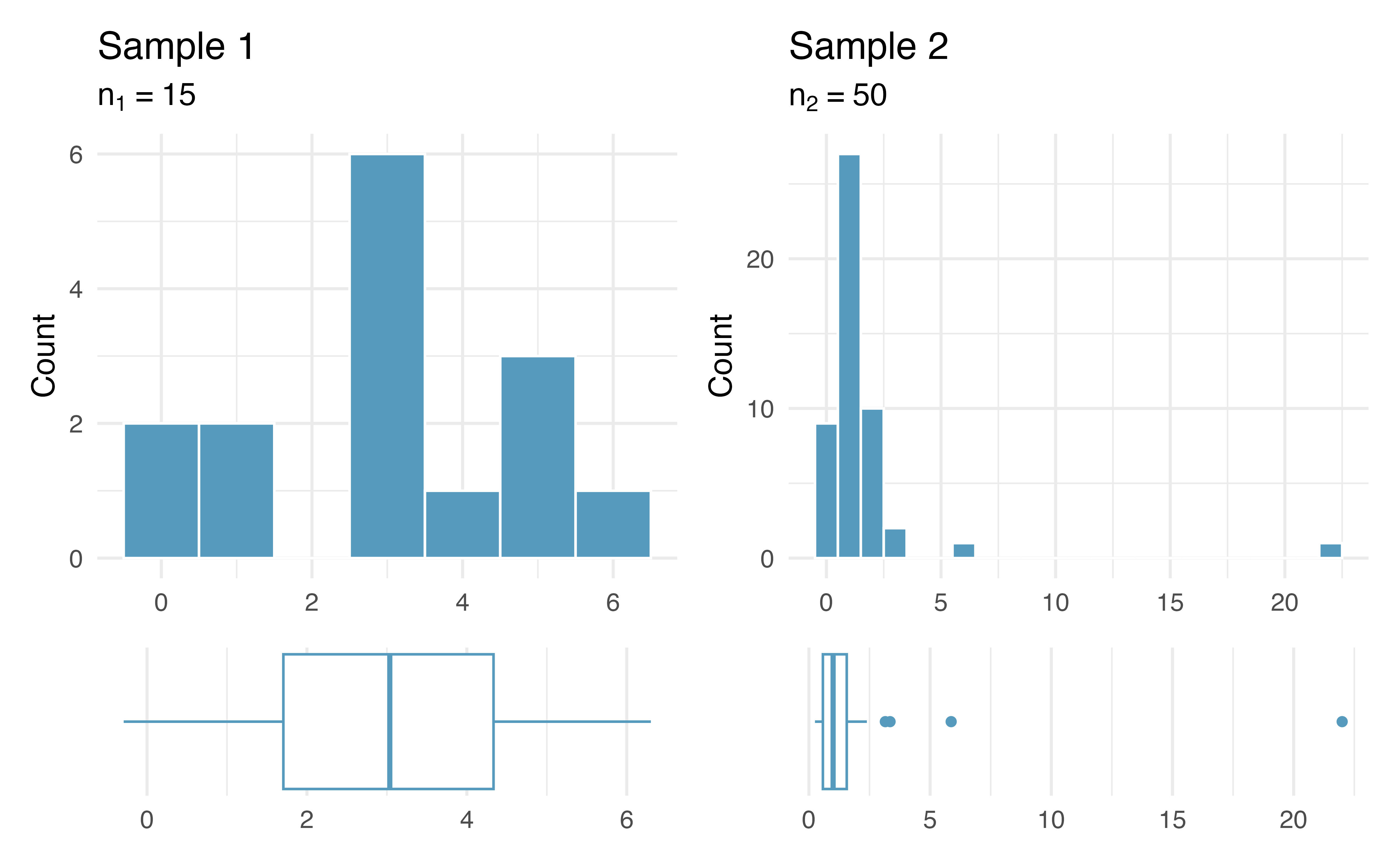
Sample 1: small \(n < 30\). But histogram and boxplot reveals no clear outliers, so I would say normality condition is met.
Sample 2: larger \(n \geq 30\). Even though \(n\) is larger, there is a particularly extreme outlier, so I would say normality condition is not met.
Height example
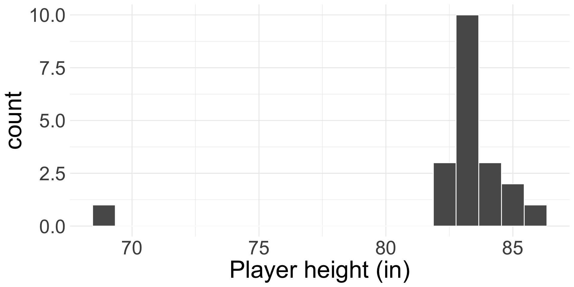
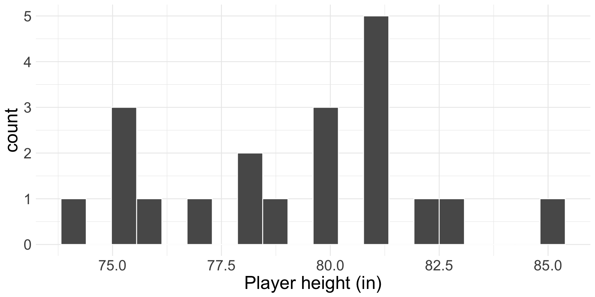
The average height of all NBA players in the 2008-9 season is 79.21 inches, with a population standard deviation of 3.57 inches. We randomly sampled 20 of these players and recorded their heights, as shown below.
What is the sampling distribution of the sample mean heights? Do we know it exactly?
The three different dists.
Note: \(y\)-axis is density (how likely each \(x\) value is from the given distribution).
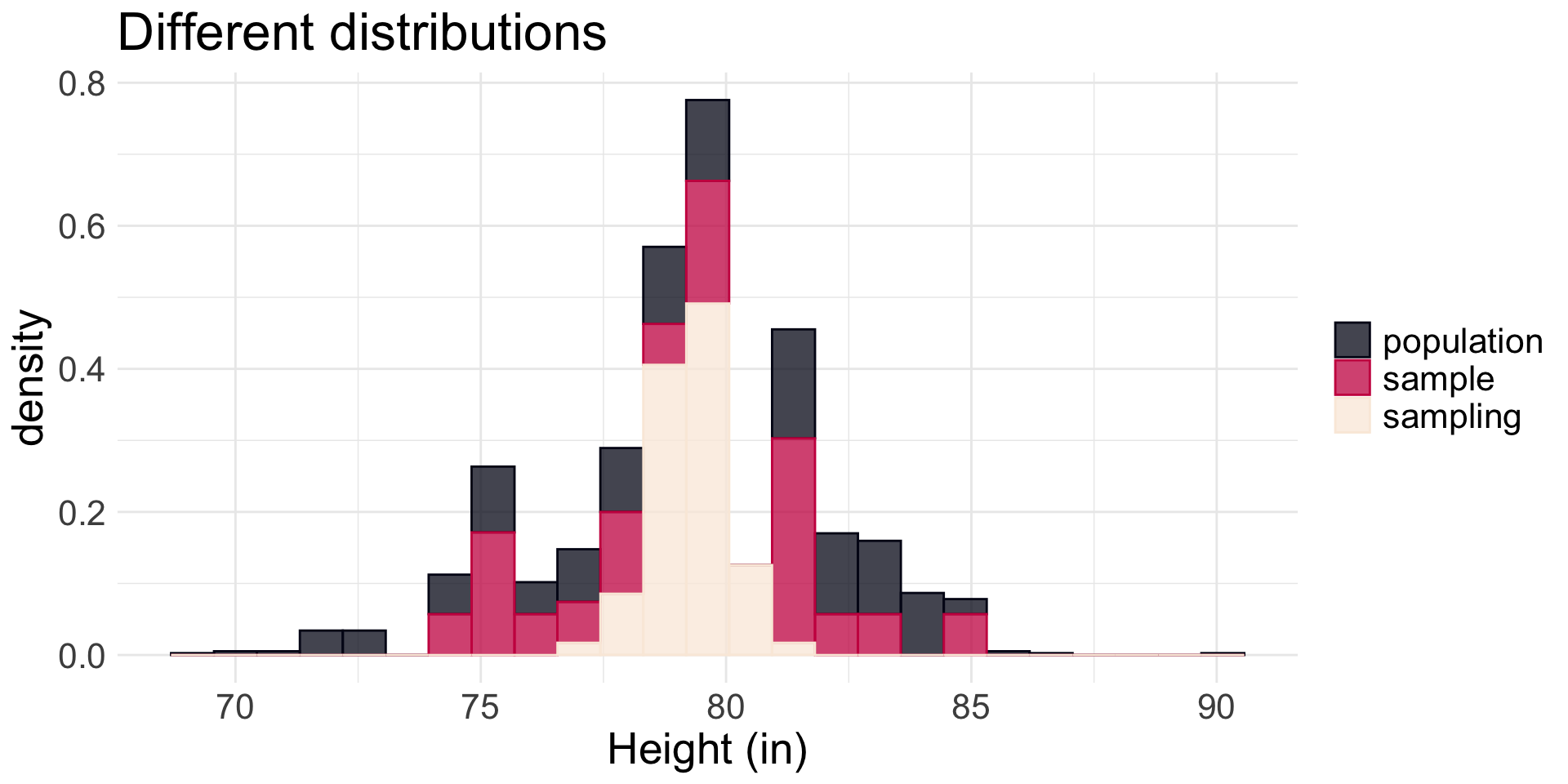
What do you notice about how the three distributions compare? Are some distributions very similar? Are some very different? Why do you think this is?
M&M’s example: solution
- Independence? Yes, due to the random sample.
- Success-failure? Depends…
If \(n= 100\):
\(np = 100(0.13) = 13 \geq 10\)
\(n(1-p) = 100(0.87) = 87 \geq 10\)
So CLT applies!
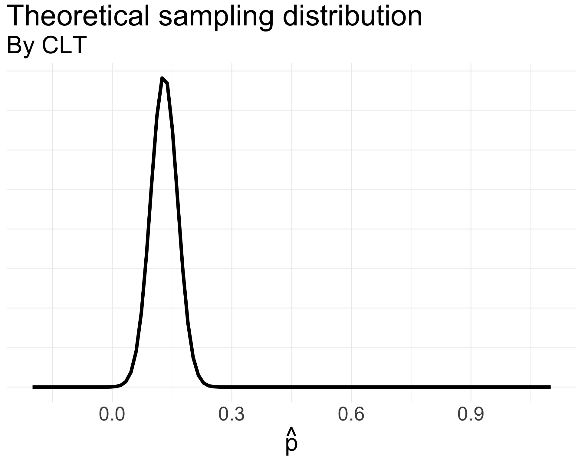
\[ \begin{align*} \hat{p} &\overset{\cdot}{\sim} N\left(0.13, \sqrt{\frac{0.13(1-0.13)}{100}}\right) \\ &= N(0.13, 0.034 ) \end{align*} \]
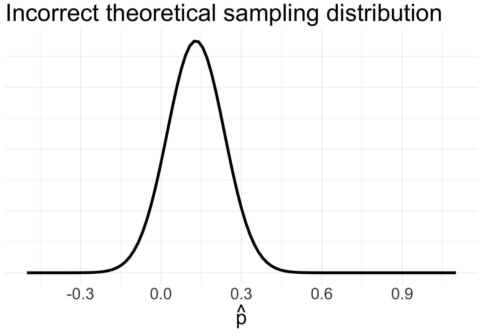
M&M’s example: solution (cont.)
- If \(n = 10\):
- \(np = 10(0.13) = 1.3 < 10\)
- Success-failure condition not met. Cannot use CLT.
If we incorrectly applied CLT, we might think \[\begin{align*} \hat{p} &\overset{\cdot}{\sim} N\left(0.13, \sqrt{\frac{0.13(1-0.13)}{10}}\right) \\ &= N(0.13, 0.106 ) \end{align*}\]
What does this distribution look like?
Why is this scary??
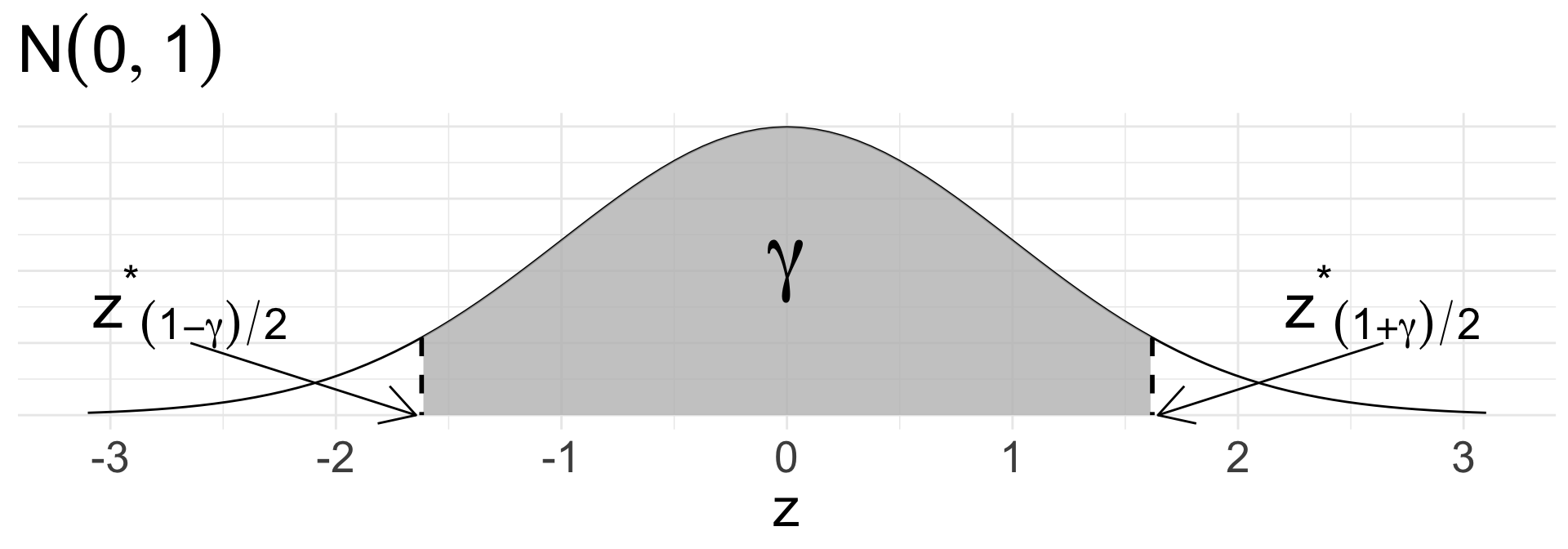
Towards a CI for a single proportion (cont.)
Critical value: to obtain the middle \(\gamma \times 100\%\), use the \(\frac{1-\gamma}{2}\) and \(\frac{1+\gamma}{2}\) percentiles of the \(N(0,1)\) distribution
\(z_{(1-\gamma)/2}^{*}\) (lower bound) and \(z_{(1+\gamma)/2}^{*}\) (upper bound)
Note: \(z_{(1+\gamma)/2}^{*} = - z_{(1-\gamma)/2}^{*}\)