CIs and HTs for a single mean

CLT-based

2025-11-03

Housekeeping

• Dessert social today! 3:30-4:30pm in WNS 105!

• Modified office hours today: 1:00-2:00pm

• Homework 7 due tonight

• Project proposals due Wednesday night at 11:59pm

Recap

• Back to numerical data

• CLT: if we have a “sufficiently large” sample of \(n\) independent observations from a population with mean \(\mu\) and standard deviation \(\sigma\), then \(\bar{X} \overset{\cdot}{\sim} N\left(\mu, \frac{\sigma}{\sqrt{n}}\right)\)

• To obtain a \(\gamma\times 100\%\) CI via CLT, we use

  \[ \text{point estimate} \pm \text{critical value} \times \text{SE} \]

  • We may need to replace the standard error with an estimate \(\widehat{SE}\)

Checking normality

• Remember, CLT requires a sufficiently large sample size \(n\) or assumption of Normality of the underlying data.

• No perfect way to check Normality, but rule of thumb:

  • If \(n < 30\) small: check that there are no clear outliers

  • If \(n \geq 30\) large: check that there are no particularly extreme outliers

CI for a single mean

If you’d like supplemental reading on CLT-based inference for a single mean: Section 19.2 of the textbook can be helpful!

CI for a single mean (known SD)

Suppose we want a \(\gamma\times 100\%\) CI for population mean \(\mu\). Also suppose that \(\sigma\) is known to us!

• If CLT holds, then we know

  \[ \bar{X} \overset{\cdot}{\sim} N\left(\mu, \frac{\sigma}{\sqrt{n}}\right) \]

• So our \(\gamma \times 100\%\) CI for \(\mu\) is:

  \[ \text{point estimate} \pm \text{critical value} \times \text{SE} = \bar{x}_{obs} \pm z_{(1+\gamma)/2}^* \times \frac{\sigma}{\sqrt{n}} \]

• Here, because we assumed \(\sigma\) known, we don’t need to (and shouldn’t) approximate \(\text{SE}\)

Example: age at marriage

In 2006-2010, the CDC conducted a thorough survey asking US women their age at first marriage. Suppose it is known that the standard deviation of the ages at first marriage is 5 years. Suppose we randomly sample 25 US women and ask them their age at first marriage (plotted below). Their average age at marriage was 23.32.

What is/are the population parameter(s)? What is the statistic?

We will obtain an 80% confidence interval for the mean age of US women at first marriage.

• Are conditions of CLT met?

• If so, what does CLT tell us?

Example: age at marriage (cont.)

Obtain an 80% confidence interval for the mean age of US women at first marriage.

• Because we have a random sample (independence) and there are no outliers in the data (normality condition), we can proceed with CLT!

\[\bar{X} \overset{\cdot}{\sim}N\left(\mu, \frac{5}{\sqrt{25}}\right) = N(\mu, 1)\]

• Construct your confidence interval and interpret!

1. Point estimate: \(\bar{x}_{obs} = 23.32\)
2. Standard error: \(\text{SE} = 1\)
3. Critical value: \(z_{0.9}^{*} =\) qnorm(0.9, 0, 1) \(= 1.28\)

So our 80% confidence interval is \(23.32 \pm 1.28 \times 1 = (22.04, 24.6)\)

Utility of this model

• The previous formula for the confidence interval for \(\mu\) relies on knowing \(\sigma\)

• But wait…

  • Want to construct a CI for \(\mu\) because we don’t know its value

  • If we don’t know \(\mu\), it seems highly unlikely that we would know \(\sigma\)!

• So in practice, we will have to estimate standard error for \(\bar{X}\):

\[ \widehat{\text{SE}} = \frac{s}{\sqrt{n}} \]

where \(s\) is the observed sample standard deviation

• Recall we did something similar for CI for \(p\), where we replaced \(p\) with \(\hat{p}_{obs}\)

Variance issue

• Estimating variance is extremely difficult when \(n\) is small, and still not great for large \(n\)

  • Replacing \(\sigma\) with \(s\) actually invalidates CLT

• So if \(\sigma\) is unknown, we cannot directly use the Normal approximation to model \(\bar{X}\) for inferential tasks

• Instead, we will use a different distribution for inference calculations, called the \(t\)-distribution

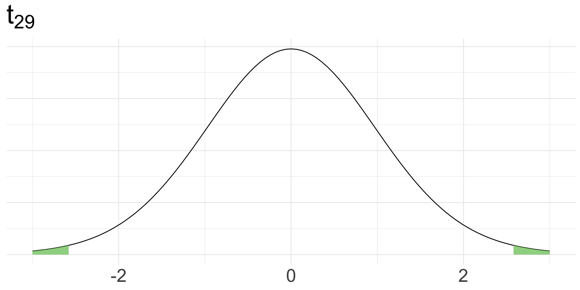
\(t\)-distribution

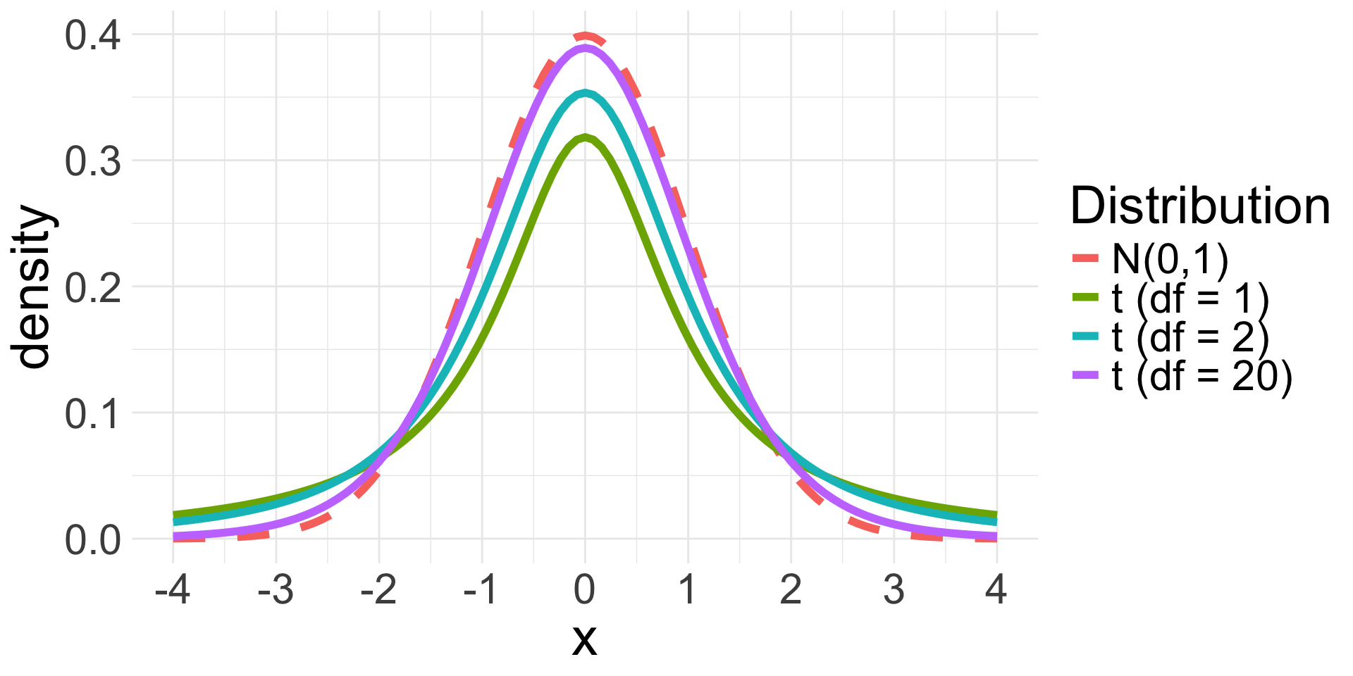
• The \(t\)-distribution is symmetric and bell-curved (like the Normal distribution)

• Has “thicker tails” than the Normal distribution (the tails decay more slowly)

• \(t\)-distribution is always centered at 0
• One parameter: degrees of freedom (df) defines exact shape of the \(t\)
  • Denoted \(t_{df}\) (e.g. \(t_{1}\) or \(t_{20}\))

• As \(df\) increases, \(t\) resembles the \(N(0,1)\). When \(df \geq 30\), the \(t_{df}\) is nearly identical to \(N(0,1)\)

\(t\) distribution in R

• pnorm(x, mean, sd) and qnorm(%, mean, sd) used to find probabilities and percentiles for the Normal distribution

• Analogous functions for \(t\)-distribution: pt(x, df) and qt(%, df)

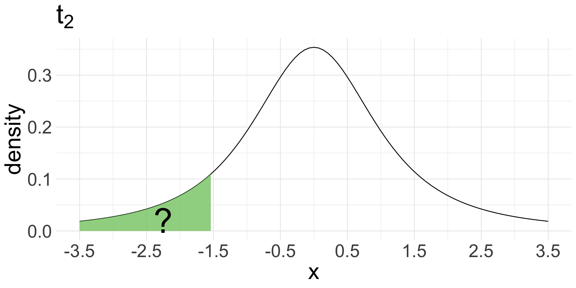
pt(-1.5,df =2) = 0.1361966

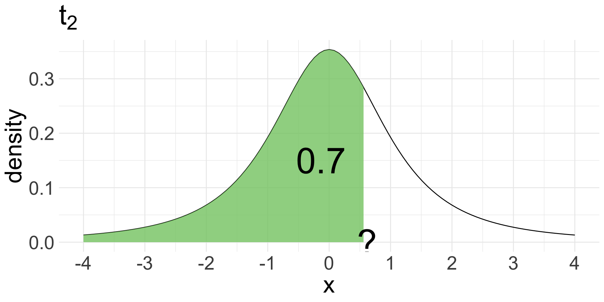
qt(0.7, df =2) = 0.6172134

CI for a single mean (unknown variance)

• Still require CLT to hold before swapping \(s\) with \(\sigma\) (independent observations and the Normality condition)

• General formula for \(\gamma \times 100\%\) CI is the same, but we simply change what goes into the margin of error.

\[ \text{point estimate} \pm t^*_{df, (1+\gamma)/2} \times \widehat{\text{SE}} = \bar{x}_{obs} \pm t_{df, (1+\gamma)/2}^* \times \frac{s}{\sqrt{n}} \]

• \(df = n-1\) (always for this CI)

• critical value \(t^*_{df, (1+\gamma)/2}\) = \((1+\gamma)/2\) percentile of the \(t_{df}\) distribution

Example: age at marriage (cont.)

Let’s return to the age at marriage example. Once again, obtain an 80% CI for the average age of first marriage for US women, but now suppose we don’t know \(\sigma\).

In our sample of \(n = 25\) women, we observed a sample mean of \(23.32\) years and a sample standard deviation of \(s = 4.03\) years.

1. Point estimate: \(\bar{x}_{obs} = 23.32\)
2. Standard error: \(\widehat{\text{SE}} = \frac{s}{\sqrt{n}}= \frac{4.03}{\sqrt{25}} = 0.806\)
3. Critical value:
   • \(df = n-1 = 24\)
   • \(t_{24, 0.9}^*\) = qt(0.9, df =24) = 1.32

So our 80% confidence interval for \(\mu\) is:

\[ 23.32 \pm 1.32 \times 0.806 = (22.26, 24.38) \]

Remarks

• Interpretation of CI does not change even if we use a different model!

• If you have access to both \(\sigma\) and \(s\), would should you use?

  • You should use \(\sigma\)!

Test for a single mean

Hypothesis test recap

1. Set hypotheses
2. Collect and summarise data, set \(\alpha\)
3. Obtain null distribution and p-value
   • For CLT-based method, obtain test statistic
4. Decision and conclusion

Hypotheses and null distribution

Want to conduct a hypothesis test for the mean \(\mu\) of a population.

• Hypotheses: \(H_0: \mu= \mu_{0}\) versus \(H_{A}: \mu \neq \mu_{0} \ (\text{or } \mu > \mu_{0} \text{ or } \mu < \mu_{0})\)

• Verify conditions for CLT

  1. Independence
  2. Approximate normality or large sample size

• Then from population with mean \(\mu\) and standard deviation \(\sigma\), we have \(\bar{X} \overset{\cdot}{\sim} N\left(\mu, \frac{\sigma}{\sqrt{n}}\right)\)

• What does the (approximate) null distribution for \(\bar{X}\) look like?

\[ \bar{X} \overset{\cdot}{\sim} N\left(\boldsymbol{\mu_{0}}, \frac{\sigma}{\sqrt{n}}\right) \]

Notice that the SE for sampling and null distribution of \(\bar{X}\) remains unchanged!

z-test and t-test statistics

Our test statistic is always of the form:

\[ \frac{\text{observed} - \text{null}}{\text{SE}_{0}} \qquad \text{ or } \qquad \frac{\text{observed} - \text{null}}{\widehat{\text{SE}}_{0}} \]

• If \(\sigma\) known and CLT met, we perform a z-test where our test-statistic is:

\[z = \frac{\bar{x}_{obs} - \mu_{0}}{\frac{\sigma}{\sqrt{n}}} \sim N(0,1)\]

and we obtain our p-value using pnorm()

• If \(\sigma\) unknown and CLT met, we perform a t-test by estimating \(\sigma\) with \(s\). Our test statistic is:

\[ t = \frac{\bar{x}_{obs} - \mu_{0}}{\frac{s}{\sqrt{n}}} \sim t_{df} \qquad df = n-1 \]

and we obtain our p-value using pt()

• Everything else proceeds as usual!

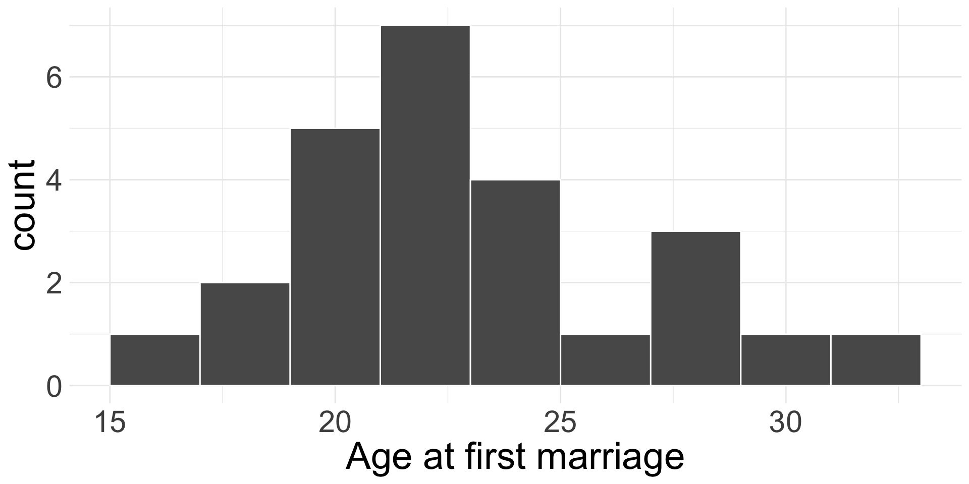
Example: salinity

The salinity level in a body of water is important for ecosystem function.

We have 30 salinity level measurements (ppt) collected from a random sample of water masses in the Bimini Lagoon, Bahamas.

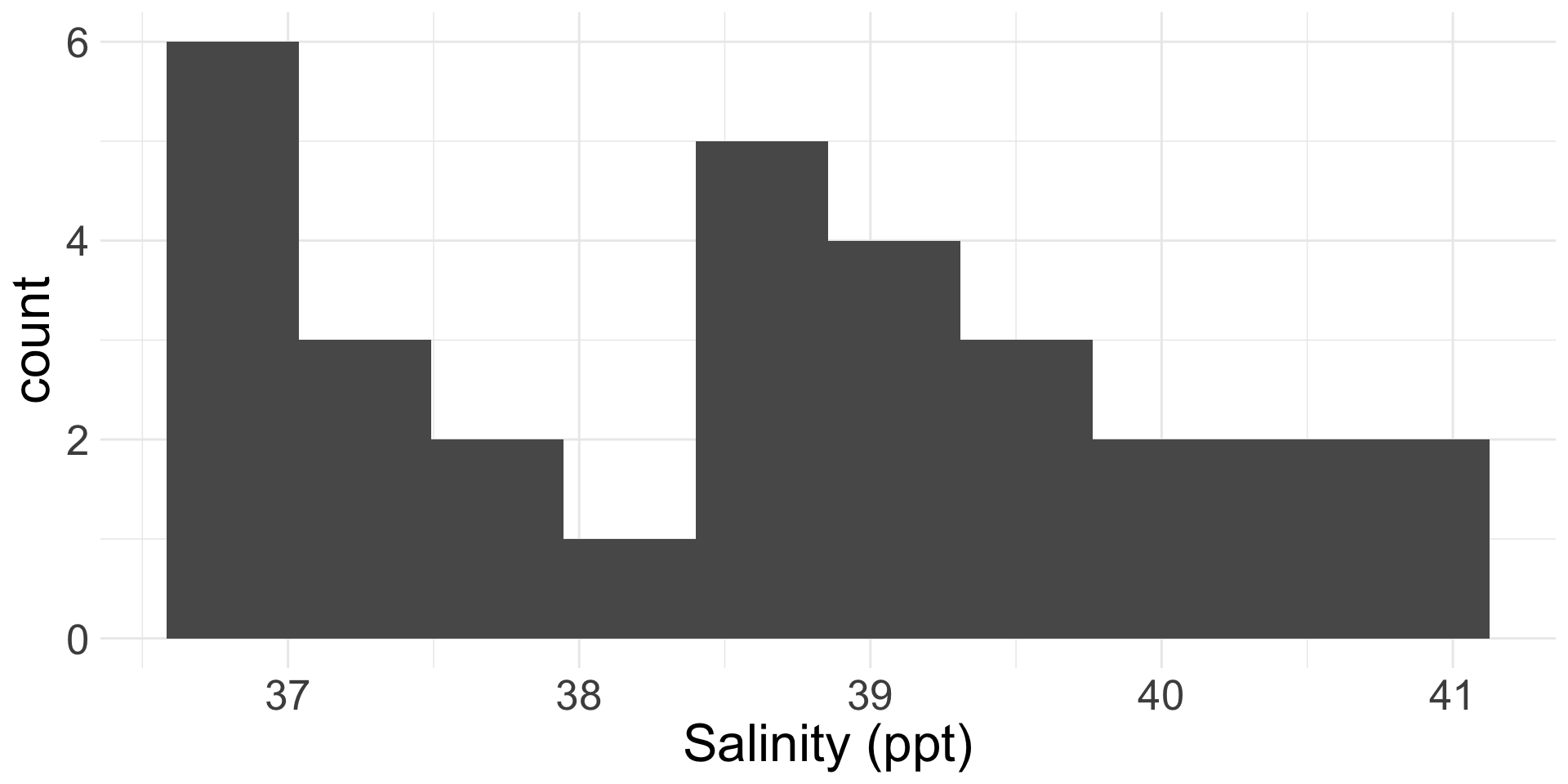
• We want to test if the average salinity level in Bimini Lagoon is different from 38 ppm at the \(\alpha = 0.05\) level.

Example: salinity (cont.)

1. Set hypotheses (define parameters as necessary).

   • Let \(\mu\) be the average salinity level in Bimini Lagoon in ppt.

   • \(H_{0}: \mu = 38\) versus \(H_{A}: \mu \neq 38\)

2. Collect summary information, set \(\alpha\).

• \(\bar{x}_{obs} = 38.6\)

• \(s = 1.29\)

• \(n = 30\)

• \(\alpha = 0.05\)

Example: salinity (cont.)

3. Obtain null distribution, test statistic, and p-value
   1. Check conditions for CLT
   2. If conditions met, obtain null distribution and test-statistic, and determine distribution of test-statistic

• Conditions:

  • Independence: random sample

  • Approximate normality: \(n = 30\), but no clear outliers

• So by CLT, null dist. is \(\bar{X} \overset{\cdot}{\sim} N\left(38, \frac{\sigma}{\sqrt{30}}\right)\)

• Since we don’t know \(\sigma\), we perform a \(t\)-test and obtain the following test-statistic:

  • \(t = \frac{\bar{x}_{obs} - \mu_{0}}{\widehat{SE}} = \frac{38.6 - 38}{1.29 / \sqrt{30}} = 2.543\)

  • This test-statistic follows a \(t_{29}\) distribution

Example: salinity (cont.)

3. Use test-statistic to obtain p-value (draw picture and/or write code using appropriate distribution)

Want \(P(T \geq 2.54) + P(T \leq 2.54)\) because \(H_{A}\) is two-sided!

p_val <- 2 * (1 - pt(t, df = n-1))
p_val

[1] 0.01658569

Example: salinity (cont.)

4. Decision and conclusion

• Since our p-value 0.017 is less than 0.05, we reject \(H_{0}\).

• The data do provide sufficient evidence to suggest that the average salinity level in Bimini Lagoon is different from 38 ppt.

Let’s code it up together!