| group | cancer | no cancer | total |
|---|---|---|---|
| control | 300 | 641 | 941 |
| herbicide | 191 | 304 | 495 |
| total | 491 | 945 | 1436 |
HTs and CIs for differences
Difference in means and proportions
2025-11-05
Housekeeping
- Project proposals due tonight!
Recap
Test and CI for a single mean if CLT applies:
If we know \(\sigma\), use \(SE = \frac{\sigma}{\sqrt{n}}\) and standard \(N(0,1)\) distribution
If we don’t know \(\sigma\), use \(\hat{SE} = \frac{s}{\sqrt{n}}\) and \(t\) distribution with \(df = n-1\)
CI for a single proportion if CLT applies:
- Use \(\hat{p}_{obs}\) in place of \(p\) to check success-failure and obtain \(\hat{SE}\)
Difference in two proportions
Now suppose we have samples of binary (e.g. success/failure) outcomes from two different populations.
Difference of two proportions
Suppose we have two populations 1 and 2, and want to either estimate the value of or conduct a test for the difference in population proportions: \(p_{1} - p_{2}\)
We have samples of size \(n_{1}\) and \(n_{2}\) from each population
Reasonable point estimate: \(\hat{p}_{1, obs} - \hat{p}_{2,obs}\)
We will obtain the sampling distribution of the difference of two sample proportions
Now that we have two populations, conditions for CLT will look slightly different!
Sampling dist. of difference of two proportions
In order to use CLT approximation for diff. in proportions, we have to ensure conditions are met:
- Independence (extended): data are independent within and between groups
- Success-failure (extended): success-failure conditions holds for both groups
- \(n_{1} p_{1} \geq 10\), \(n_{1} (1-p_{1}) \geq 10\), \(n_{2} p_{2} \geq 10\), and \(n_{2} (1-p_{2}) \geq 10\)
If above hold, then:
\[ \hat{p}_{1} - \hat{p}_{2} \overset{\cdot}{\sim} N\left(p_{1} - p_{2}, \sqrt{\frac{p_{1} (1-p_{1})}{n_{1}} + \frac{p_{2} (1-p_{2})}{n_{2}}} \right) \]
where \(p_{1}\) and \(p_{2}\) are the population proportions
Confidence interval for difference in proportions
If we want to obtain a \(\gamma\times 100\%\) CI for \(p_{1} - p_{2}\), that means we don’t know the value of \(p_{1} - p_{2}\)!
Like in the case of the CI for a single proportion, we will use our observed proportions to check success-failure
Success-failure condition for CI for difference in proportions:
\(n_{1} \hat{p}_{1,obs} \geq 10\) and \(n_{1} (1-\hat{p}_{1,obs}) \geq 10\)
\(n_{2} \hat{p}_{2,obs} \geq 10\) and \(n_{2} (1-\hat{p}_{2,obs}) \geq 10\)
Then our formula for the CI is the same as before:
\[ \begin{align*} &\text{point. est} \pm \text{critical val.}\times \widehat{\text{SE}} = \\ &(\hat{p}_{1,obs} - \hat{p}_{2,obs}) \pm z^{*}_{(1+\gamma)/2} \sqrt{\frac{\hat{p}_{1,obs} (1-\hat{p}_{1,obs})}{n_{1}} + \frac{\hat{p}_{2,obs} (1-\hat{p}_{2,obs})}{n_{2}}} \end{align*} \]
Diff. props CI example: cancer in dogs
A study in 1994 examined over 1400 randomly sampled dogs, some of which had been exposed to the herbicide 2,4-Dichlorophenoxyacetic acid. They wanted to do know if there is an increased risk in dogs in developing cancer due to exposure to 2,4-D. We have the following data:
Let’s obtain a 95% CI via the CLT for the difference in the rate cancer outcomes between dogs exposed to 2,4-D and dogs not exposed to the herbicide.
Diff. props CI example (cont.)
Let population 1 be dogs exposed to 2,4-D, and population 2 be dogs not exposed to 2,4-D. We want a 95% CI for \(p_{1} - p_{2}\), where \(p_{i}\) is the rate of cancer in population \(i\).
Obtain useful statistics
\(n_{1} = 495\), \(n_{2} = 941\)
\(\hat{p}_{1, obs} = \frac{191}{495} = 0.386\)
\(\hat{p}_{2, obs} = \frac{300}{941} = 0.319\)
Check conditions for CLT.
Independence (extended)? Randomly sampled
Success-failure (extended)?
- \(n_{1}\hat{p}_{1,obs} = 191 \geq 10\)
- \(n_{1}(1-\hat{p}_{1,obs}) = 304 \geq 10\)
- \(n_{2}\hat{p}_{2,obs} = 300 \geq 10\)
- \(n_{2}(1-\hat{p}_{2,obs}) = 641 \geq 10\)
- Since both conditions are met, we can proceed with the CLT.
Diff. props CI example (cont.)
Collect the components of CI:
Point estimate
Critical value (code)
\(\text{SE}\) or \(\widehat{\text{SE}}\)
\(\hat{p}_{1,obs} - \hat{p}_{2,obs} = 0.386 - 0.319 = 0.067\)
\(z^{*}_{0.975} =\)
qnorm(0.975, 0, 1)\(\approx 1.96\)\(\widehat{\text{SE}} = \sqrt{\frac{0.386(1 - 0.386)}{495} + \frac{0.319(1 - 0.319)}{941}} = 0.027\)
So putting it all together, our 95% CI is:
\[ 0.067 \pm 1.96 \times 0.027 = (0.014, 0.12) \]
Interpret!
- We are 95% confident the that the true difference in rates of cancer among dogs exposed to 2,4-D and dogs not exposed to 2,4-D is between 0.014 and 0.12 (exposed - control).
Hypothesis test for difference in proportions
Recall, hypothesis tests for differences take the form:
\[\begin{align*} H_{0}:\ p_{1} - p_{2} &= 0 \\ H_{A}: \ p_{1} - p_{2} &\neq 0 \qquad (\text{ or } > \qquad \text{ or } <) \end{align*}\]
To use CLT, need independence (extended) and success-failure condition under \(H_{0}\) (extended)
Unlike before, we don’t have specific null-hypothesized values for \(p_{1}\) or \(p_{2}\).
So how do we check the success-failure condition??
Pooled proportion
Since \(H_{0}: p_{1} = p_{2}\), then under the null \(\hat{p}_{1,obs}\) and \(\hat{p}_{2,obs}\) come from the same population
So under this null, we use a special proportion called the pooled proportion:
\[ \hat{p}_{pooled} = \frac{\text{total # of successes from both samples}}{\text{combined sample size}} \]
This is the best estimate of both \(p_{1}\) and \(p_{2}\) if \(H_{0}: p_{1} = p_{2}\) is true! Thus putting us in \(H_{0}\)
- For this reason, use \(\hat{p}_{pooled}\) to verify success-failure conditions for HT for difference of proportions:
- \(n_{1} \hat{p}_{pooled} \geq 10\) and \(n_{1} (1-\hat{p}_{pooled}) \geq 10\)
- \(n_{2} \hat{p}_{pooled} \geq 10\) and \(n_{2} (1-\hat{p}_{pooled}) \geq 10\)
Hypothesis test (cont.)
- Obtain null distribution
- If conditions satisfied, then we know the sampling distribution of \(\hat{p}_{1} - \hat{p}_{2}\)
- To obtain the null distribution we assume \(H_{0}: p_{1} - p_{2} = 0\) is true and we \(\hat{p}_{pooled}\) to estimate \(p_{1}\) and \(p_{2}\) to approximate standard error under the null:
\[\begin{align*} \hat{p}_{1} - \hat{p}_{2} &\overset{\cdot}{\sim} N\left(p_{1} - p_{2}, \sqrt{\frac{p_{1} (1-p_{1})}{n_{1}} + \frac{p_{2} (1-p_{2})}{n_{2}}} \right) \qquad \text{(CLT)} \\ &\overset{\cdot}{\sim} N\big(0, \sqrt{\frac{\hat{p}_{pooled}(1 - \hat{p}_{pooled})}{n_{1}} + \frac{\hat{p}_{pooled}(1 - \hat{p}_{pooled})}{n_{2}}} \big) \qquad (H_{0}) \end{align*}\]
- This last square root is \(\widehat{SE}_{0}\), our approximate standard error under \(H_{0}\)
Hypothesis test (cont.)
Obtain test-statistic:
\[ z = \frac{\text{point estimate} - \text{null value}}{\text{SE}_{0}} \approx \frac{(\hat{p}_{1,obs} - \hat{p}_{2,obs}) - 0}{\widehat{\text{SE}}_{0}} \]
To obtain p-value, we want \(\text{Pr}(Z \geq z)\) and/or \(\text{Pr}(Z \leq z)\) where \(Z \sim N(0,1)\)
- As before, obtain using
pnorm(z, 0, 1)
- As before, obtain using
Diff. props HT example: cancer in dogs (again)
Using the same data as before, let’s answer the following question:
Do the data provide strong evidence at the 0.05 level that the rate of cancer is higher for dogs exposed to 2,4-D than that of dogs not exposed to the herbicide?
Let \(p_{1}\) and \(p_{2}\) be defined as before.
Define hypotheses
- \(H_{0}: p_{1} - p_{2} = 0\) and \(H_{A}: p_{1} - p_{2} > 0\)
Diff. props HT example (cont.)
Obtain pooled proportion, and use it to check conditions for CLT.
\(\hat{p}_{pooled} =\frac{191 + 300}{495 + 941} = \frac{491}{1436} = 0.342\)
Conditions
Independence (extended): random sample
Success-failure (extended):
\(n_{1} \hat{p}_{pooled} = 495 \times 0.342 = 169.29 \geq 10\)
\(n_{1} (1 - \hat{p}_{pooled}) = 495 \times (1 - 0.342) = 325.71 \geq 10\)
\(n_{2} \hat{p}_{pooled} = 941 \times 0.342 = 321.82 \geq 10\)
\(n_{2} (1 - \hat{p}_{pooled}) = 941 \times (1 - 0.342) = 619.18 \geq 10\)
Since conditions are met, we can proceed with CLT-based test!
Diff. props HT example (cont.)
Find the null distribution for \(\hat{p}_{1} - \hat{p}_{2}\).
\[ \hat{p}_{1} - \hat{p}_{2} \overset{\cdot}{\sim}N\left(0, \sqrt{\frac{0.342(1 - 0.342)}{495} + \frac{0.342(1 - 0.342)}{941}} = 0.026 \right) \]
Set up calculation for test statistic
\[ z =\frac{( \hat{p}_{1, obs}- \hat{p}_{2, obs}) - 0}{\widehat{\text{SE}}_{0}} = \frac{(0.386 - 0.319) - 0}{0.026} = 2.577 \]
Diff. props HT example (cont.)
Draw picture and write code for p-value
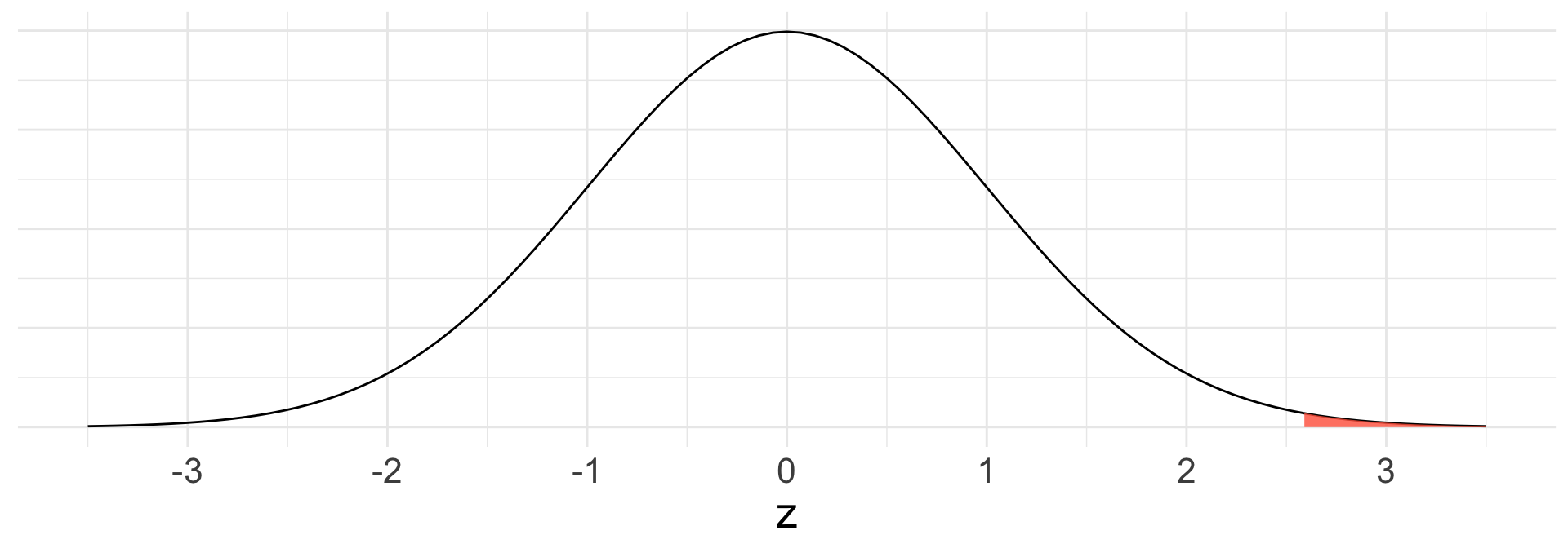
p-value calculation:
\(\text{Pr}(Z \geq z) = \text{Pr}(Z \geq 2.577)\)
1 - pnorm(2.577, 0, 1)= 0.0049831
Make a decision and conclusion in context.
- Since our p-value is less than 0.05, we reject \(H_{0}\). The data do provide strong evidence that dogs exposed to 2,4-D have higher rates of cancer than dogs not exposed to the herbicide.
Difference in two means
Difference in two means
We still have two populations, but the variable of interest is quantitative (i.e. not binary).
We are interested in learning about the difference in the means of each population.
Let \(\mu_{1}\) and \(\mu_{2}\) represent the population means for the two populations 1 and 2
Samples of size \(n_{1}\) and \(n_{2}\) from each population, respectively
Conditions for CLT
Independence (extended): need data within and between the two groups
- e.g.the two data sets come from independent random samples or from a randomized experiment
Normality: we need to check for approximate normality for both groups separately
CLT for difference in two sample means
If CLT conditions met, the distribution of difference in sample means is:
\[ \bar{X}_{1} - \bar{X}_{2} \overset{\cdot}{\sim} N\left(\mu_{1} - \mu_{2}, \sqrt{\frac{\sigma_{1}^2}{n_{1}} + \frac{\sigma_{2}^2}{n_{2}}} \right) \] where \(n_{1}\) and \(n_{2}\) are the sample sizes.
- Remember, we often do not know \(\sigma_{1}\) nor \(\sigma_{2}\)
- In practice, will have to estimate with \(s_{1}\) and \(s_{2}\) and use the \(t\)-distribution
CI for difference in two means
If the conditions hold, then our usual formula for \(\gamma \times 100\%\) CI still holds:
\[ \text{point estimate} \pm \text{critical value} \times \text{SE} \]
Point estimate: \(\bar{x}_{1,obs} - \bar{x}_{2,obs}\)
If \(\sigma_{1}\) and \(\sigma_{2}\) known:
\(\text{SE} = \sqrt{\frac{\sigma_{1}^2}{n_{1}} + \frac{\sigma_{2}^2}{n_{2}}}\)
Critical value: \(z_{(1+\gamma)/2}^*\)
- \((1+\gamma)/2\) percentile of \(N(0,1)\)
If \(\sigma_{1}\) and \(\sigma_{2}\) unknown:
\(\widehat{\text{SE}} \approx \sqrt{\frac{s_{1}^2}{n_{1}} + \frac{s_{2}^2}{n_{2}}}\)
critical value: \(t_{df, (1+\gamma)/2}^*\)
\((1+\gamma)/2\) percentile of \(t_{df}\)
\(df = \min\{n_{1} -1, n_{2} - 1\}\)
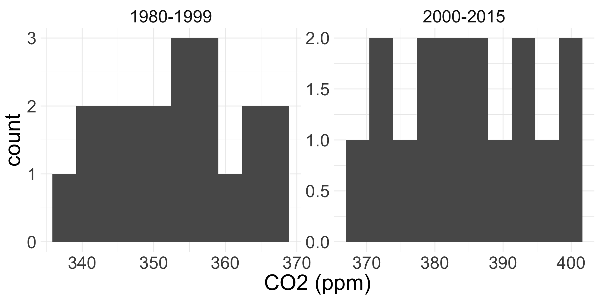
Diff. means CI example: C02 concentrations
The Mauna Loa Observatory in Hawaii of monitors atmospheric solar, atmospheric, and meteorological parameters
We have data on annual atmospheric CO2 concentrations from 1980-2015.
We will obtain a 90% confidence interval for the difference between the average atmospheric C02 levels (ppm) from years 2000-2015 and years 1980-1999.
| group | n | xbar | s |
|---|---|---|---|
| 1980-1999 | 20 | 353.12 | 9.0 |
| 2000-2015 | 16 | 385.02 | 9.9 |
Diff. means CI example (cont.)
Define parameters.
- Let \(\mu_{1}\) be the average CO2 levels from 2000-2015 and \(\mu_{2}\) the average CO2 levels from 1980-1999.
- Want to obtain a 90% CI for \(\mu_{1} - \mu_{2}\)
- Note: could also do \(\mu_{2} - \mu_{1}\) (interpretation just changes slightly)
Check conditions for CLT.
Independence (extended): most likely violated because CO2 levels are probably dependent across time. BUT let’s proceed with caution anyway.
Normality: \(n_{1} = 16 < 30\) and \(n_{2} = 20 < 30\). But since histograms don’t reveal outliers, Normality condition appears met.
Diff. means CI example (cont.)
Collect components for CI:
Point estimate
Critical value (code)
\(\text{SE}\) or \(\widehat{\text{SE}}\)
\(\bar{x}_{1,obs} - \bar{x}_{2,obs} = 385.02 - 353.12 = 31.9\)
Since we don’t know \(\sigma_{1}\) nor \(\sigma_{2}\), need to use \(t\)-distribution
Degrees of freedom = \(\min\{16 - 1, 20 -1\} = 15\)
\(t^*_{0.95}\) =
qt(0.95, df = 15)= 1.75
\(\widehat{\text{SE}} = \sqrt{\frac{9.9^2}{16} + \frac{9^2}{20}} = 3.19\)
Put it all together:
\[ \text{point est.} \pm \text{crit. val}\times \text{SE} = 31.9 \pm 1.75 \times 3.19 = (26.3175, 37.4825) \]
Diff. means CI example (cont.)
Interpret our CI of (26.3175, 37.4825) in context!
Hypothesis test for difference in means
Now suppose we’re interested in testing for the difference between \(\mu_{1}\) and \(\mu_{2}\).
\(H_{0}: \mu_{1} - \mu_{2} = 0\) versus \(H_{A}: \mu_{1} - \mu_{2} \neq 0\) (or \(<\) or \(>\))
Same conditions as in CI are necessary for CLT-based inference!
- Independence (extended)
- Normality condition for both groups
If CLT met, then under \(H_{0}\), the null distribution is
\[ \bar{X}_{1} - \bar{X}_{2} \overset{\cdot}{\sim} N\left(0, \sqrt{\frac{\sigma_{1}^2}{n_{1}} + \frac{\sigma_{2}^2}{n_{2}}} \right) \]
Test statistic for difference in means
Test-statistic is of form:
\[ \frac{\text{point est.} - \text{null value}}{\text{SE}_{0}} \]
If \(\sigma_{1}, \sigma_{2}\) known, our test-statistic is:
\[ z = \frac{(\bar{x}_{1,obs} - \bar{x}_{2,obs}) - 0}{ \sqrt{\frac{\sigma_{1}^2}{n_{1}} + \frac{\sigma_{2}^2}{n_{2}}}} \sim N(0,1) \]
If \(\sigma_{1}, \sigma_{2}\) unknown, our test-statistic is
\[ t = \frac{(\bar{x}_{1,obs} - \bar{x}_{2,obs}) - 0}{ \sqrt{\frac{s_{1}^2}{n_{1}} + \frac{s_{2}^2}{n_{2}}}} \sim t_{df} \]
\(df = \min\{n_{1}-1, n_{2}-1 \}\)
Diff. means HT example: CO2
Now let’s test if the mean CO2 level in 2000-2015 was greater than that mean CO2 level in 1980-1999 at the \(0.05\) level using CLT.
- \(H_{0}: \mu_{1} - \mu_{2} = 0\) versus \(H_{A}: \mu_{1} - \mu_{2} > 0\), where \(\mu_{1}\) and \(\mu_{2}\) were defined previously
- Let \(\alpha = 0.05\)
- Conditions for CLT are same as before (proceed with caution)
Diff. means HT example (cont.)
Obtain test-statistic and p-value.
Find the value of the test-statistic and its distribution
\[ t = \frac{(385.02 - 353.12)- 0}{3.19} = 10 \sim t_{15} \]
Write code for p-value (optionally draw picture)
- p-value =
1 - pt(10, df = 15)= 0 (tiny!)