| x | y | y_hat | residual |
|---|---|---|---|
| -2.991 | 2.481 | -0.130 | 2.611 |
| -1.005 | -1.302 | 0.691 | -1.994 |
| 3.990 | 3.929 | 2.757 | 1.172 |
Introduction to Simple Linear Regression
2025-11-10
Linear relationship
Suppose we have the following data:
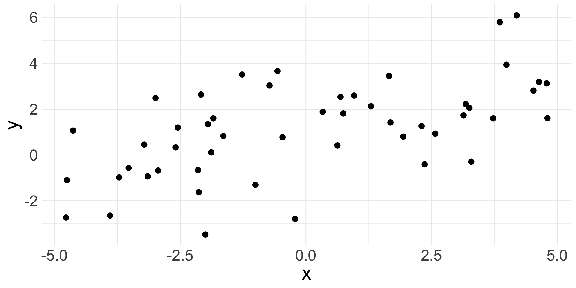
- Observations won’t fall exactly on a line, but do fall around a straight line, so maybe a linear relationship makes sense!
Fitted values (cont.)
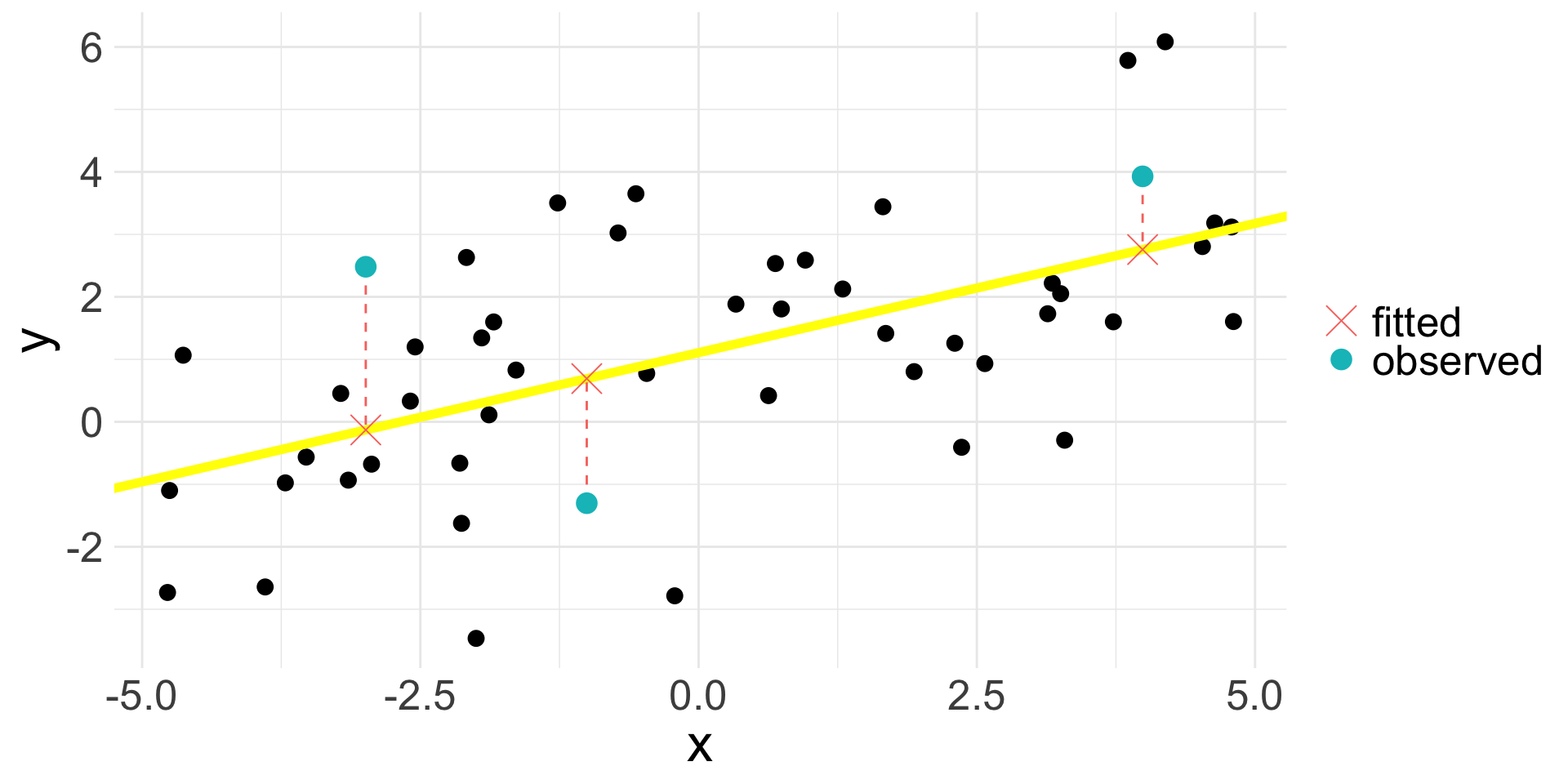
- Suppose our estimated line is the yellow one: \(\hat{y} = 1.11 + 0.41 x\)
- The fitted value \(\hat{y}_{i}\) for \(y_{i}\) lies on the line; the above plot shows three specific examples
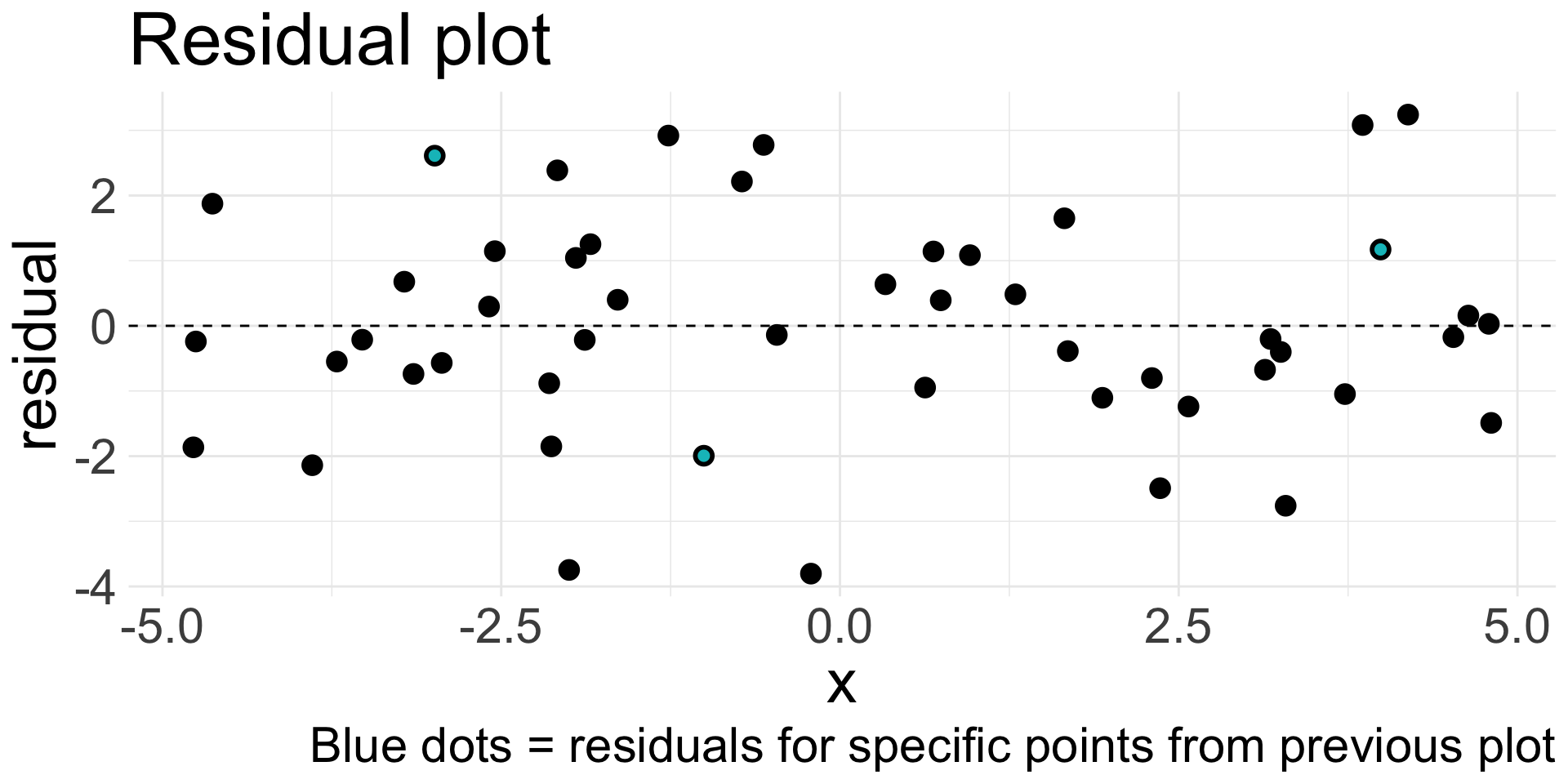
Residual (cont.)

Residual values for the three highlighted observations:
Residual plot
Residuals are very helpful in evaluating how well a model fits a set of data
Residual plot: original \(x\) values plotted against corresponding residuals on \(y\)-axis
Residual plot (cont.)
Residual plots can be useful for identifying characteristics/patterns that remain in the data even after fitting a model.
Just because you fit a model to data, does not mean the model is a good fit!
Can you identify any patterns remaining in the residuals?
Describing linear relationships
Different data may exhibit different strength of linear relationships:
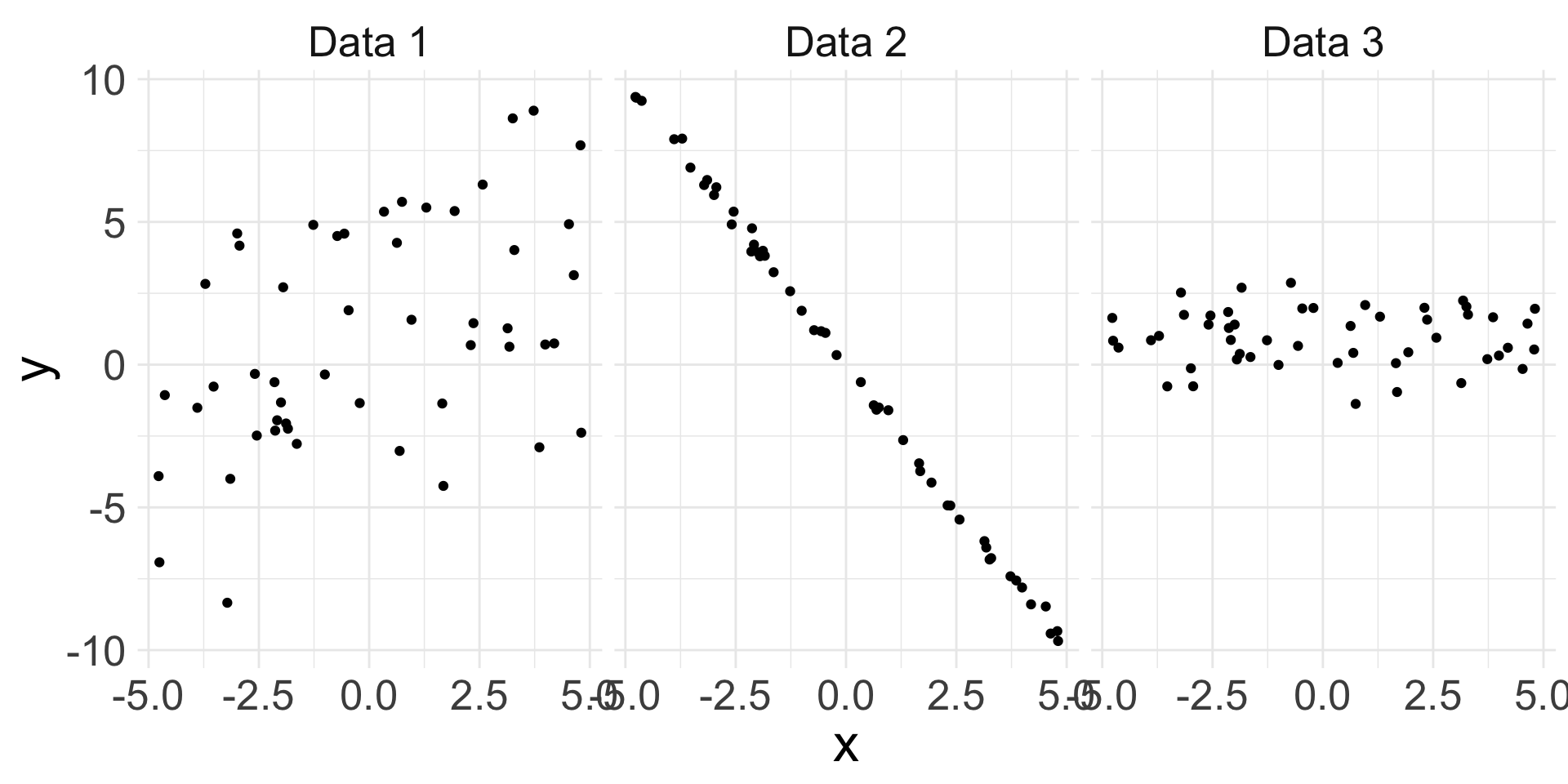
- Can we quantify the strength of the linear relationship?
Correlation
Correlation is describes the strength of a linear relationship between two variables
- The observed sample correlation is denoted by \(R\)
- Formula (not important): \(R = \frac{1}{n-1} \sum_{i=1}^{n} \left(\frac{x_{i} - \bar{x}}{s_x} \right)\left(\frac{y_{i} - \bar{y}}{s_y} \right)\)
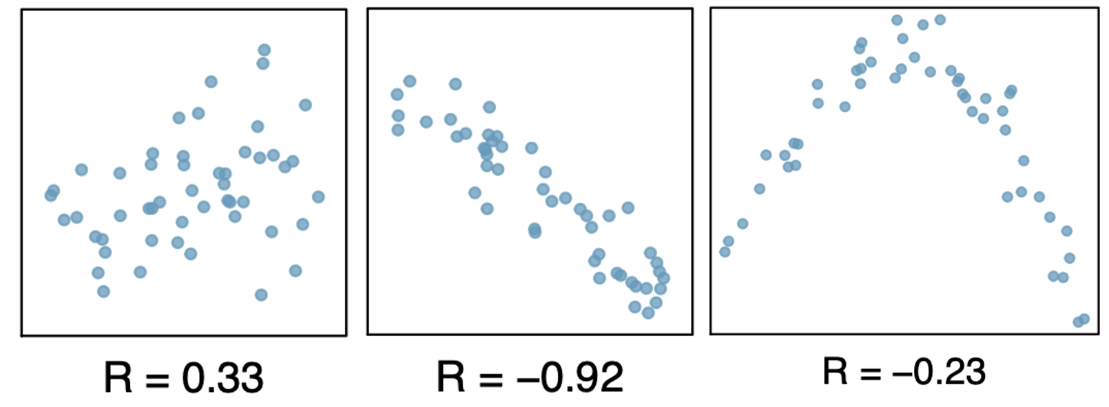
Always takes a value between -1 and 1
-1 = perfectly linear and negative
1 = perfectly linear and positive
0 = no linear relationship
Nonlinear trends, even when strong, sometimes produce correlations that do not reflect the strength of the relationship
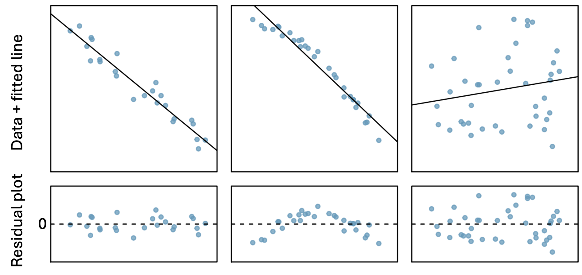
Different lines
The following display the same set of 50 observations.
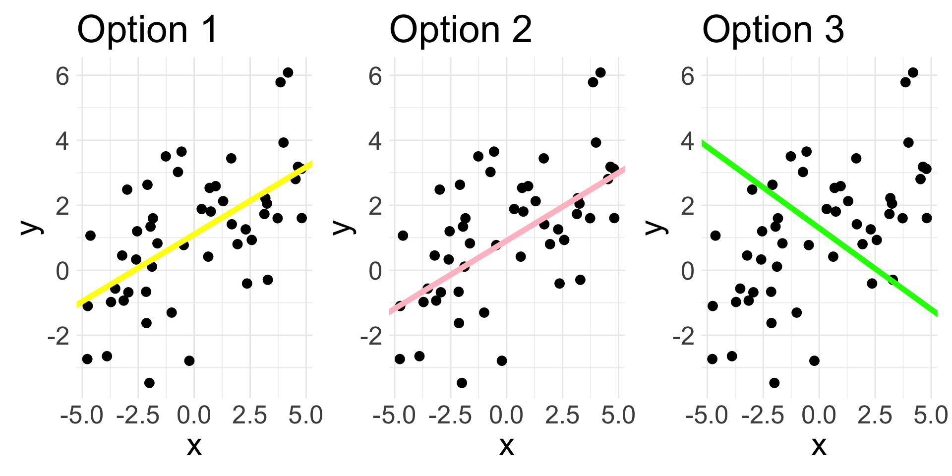
Which line would you say fits the data the best?
There are infinitely many choices of \((b_{0}, b_{1})\) that could be used to create a line
We want the BEST choice (i.e. the one that gives us the “line of best fit”)
How to define “best”?
1. Linearity
Assess before fitting the linear regression model by making a scatterplot of \(x\) vs. \(y\):
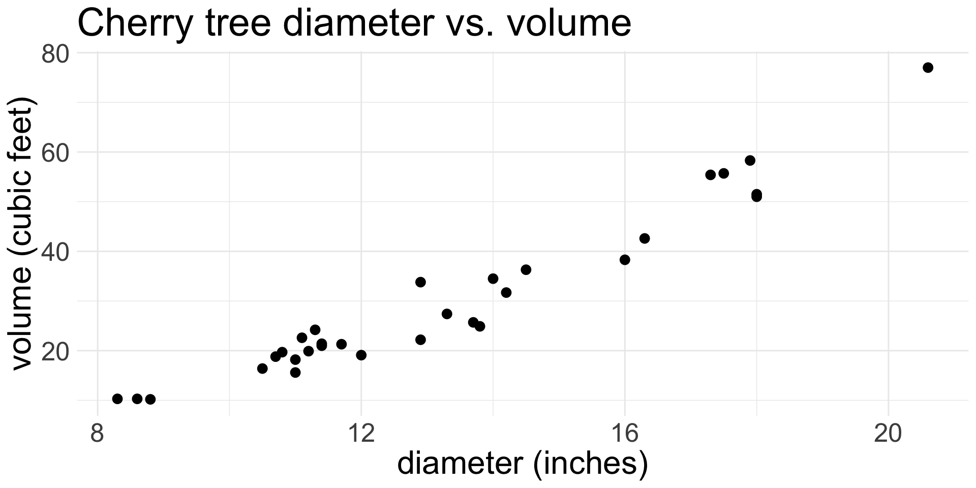
Does there appear to be a linear relationship between diameter and volume?
- I would say yes
2. Independence
Assess before fitting the linear regression model by understanding how your data were sampled.
- The
cherrydata do not explicitly say that the trees were randomly sampled, but it might be a reasonable assumption
An example where independence is violated:
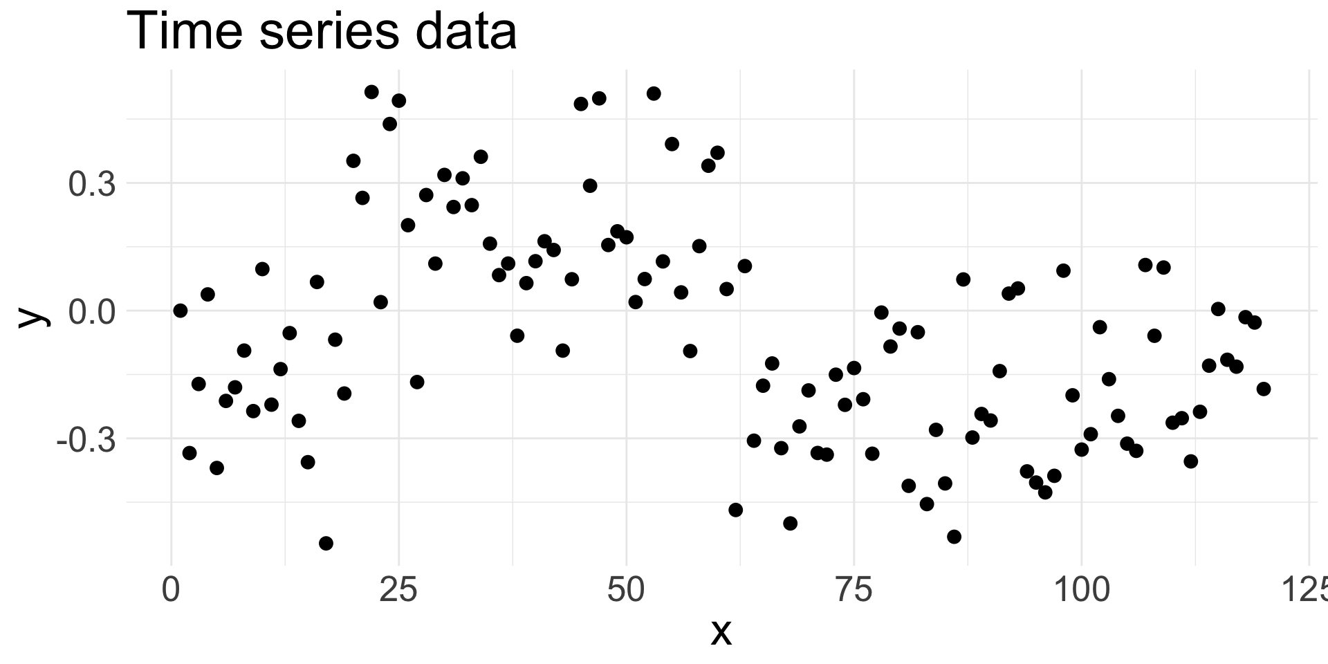
Here, the data are a time series, where observation at time point \(i\) depends on the observation at time \(i-1\).
- Successive/consecutive observations are highly correlated
3. Nearly normal residuals
Assess after fitting the model by making histogram of residuals and checking for approximate Normality.
- Remember, residuals are \(e_{i} = y_{i} - \hat{y}_{i}\)
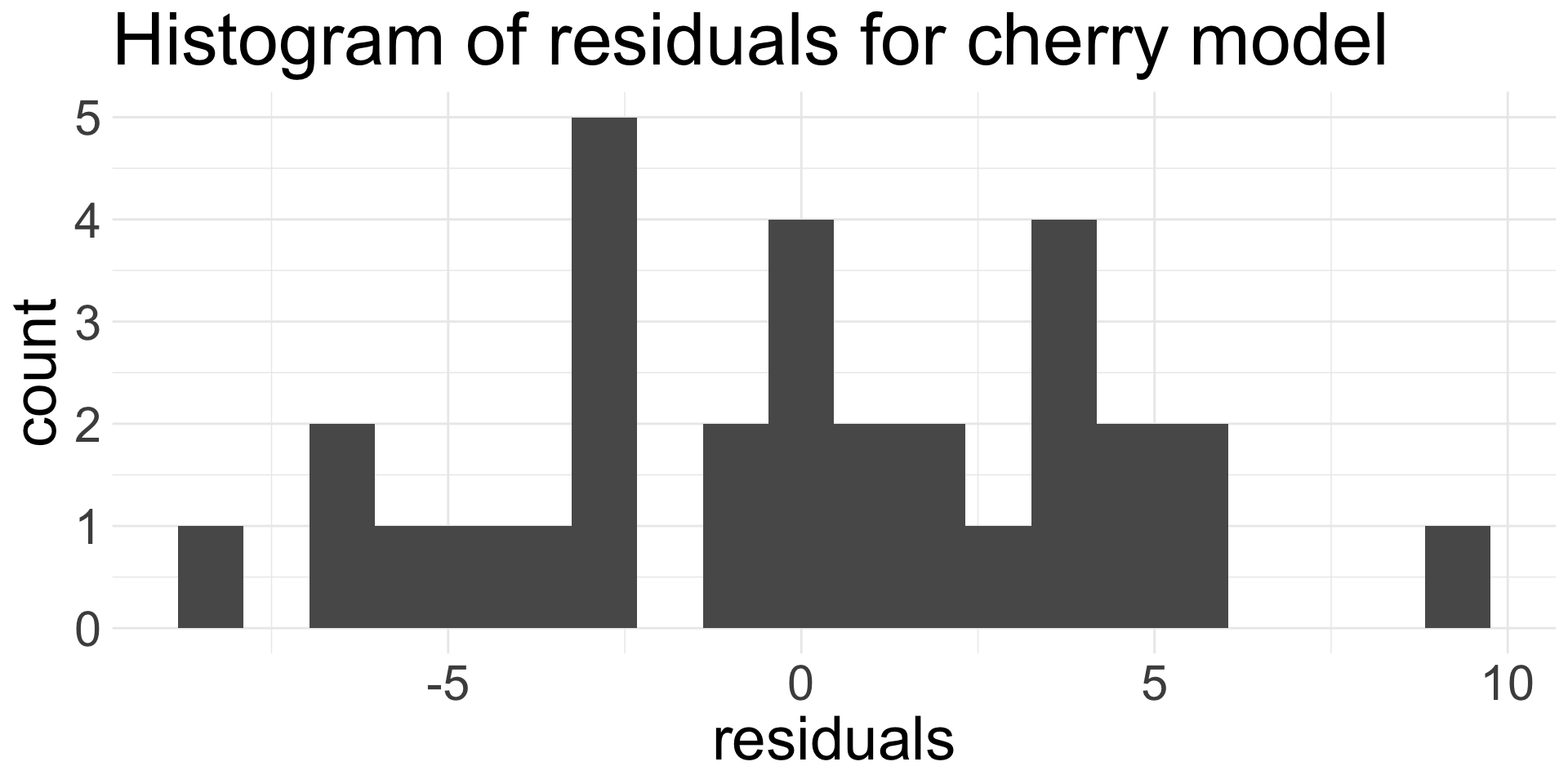
Do the residuals appear approximately Normal?
- I think so!
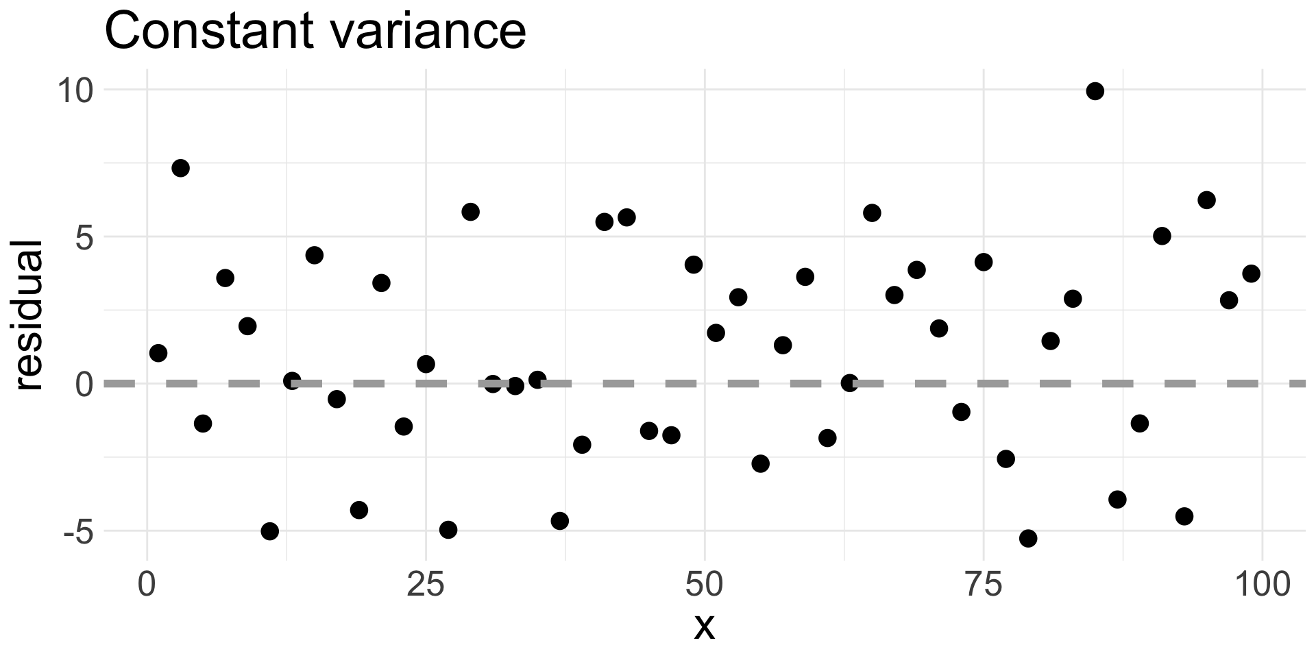
4. Equal variance
Assess after fitting the model by examining a residual plot and looking for patterns.
A good residual plot:
A bad residual plot:
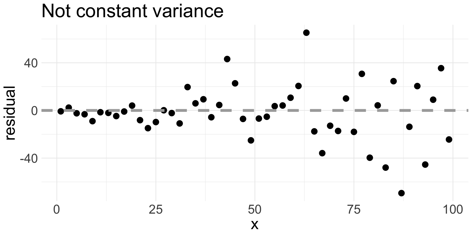
We usually add a horizontal line at 0.
4. Equal variance (cont.)
Let’s examine the residual plot of our fitted model for the cherry data:
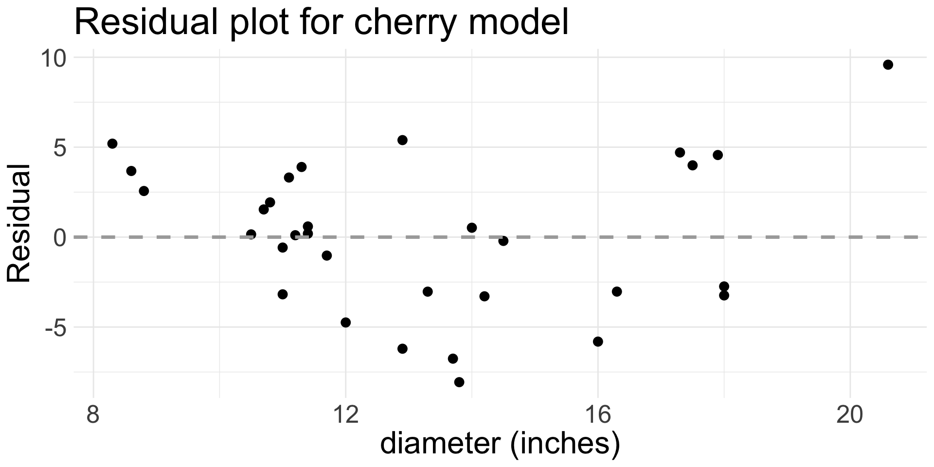
Do we think equal variance is met?
I would say there is a definite pattern in the residuals, so equal variance condition is not met.
Some of the variability in the errors appear related to
diameter