Inference in SLR
2025-11-13
Housekeeping
Midterm 2 is one week from today (in class)
- Practice problems to be released over the weekend
Coding practice due tonight
Recap
- Learned how to interpret slope and intercept of fitted model
- \(b_0\) is estimate of \(\hat{y}\) when \(x=0\)
- \(b_{1}\) is expected change in \(\hat{y}\) for a one unit increase in \(x\)
- When explanatory \(x\) is categorical, we have a slightly more nuanced interpretation
- Created indicator variable with 0 = base level and 1 = non-base level
- Coefficient of determination \(R^2\) assesses strength of linear model fit
Live code!
How to fit a sample linear regression model in R. (Code posted after class!)
Inference for SLR
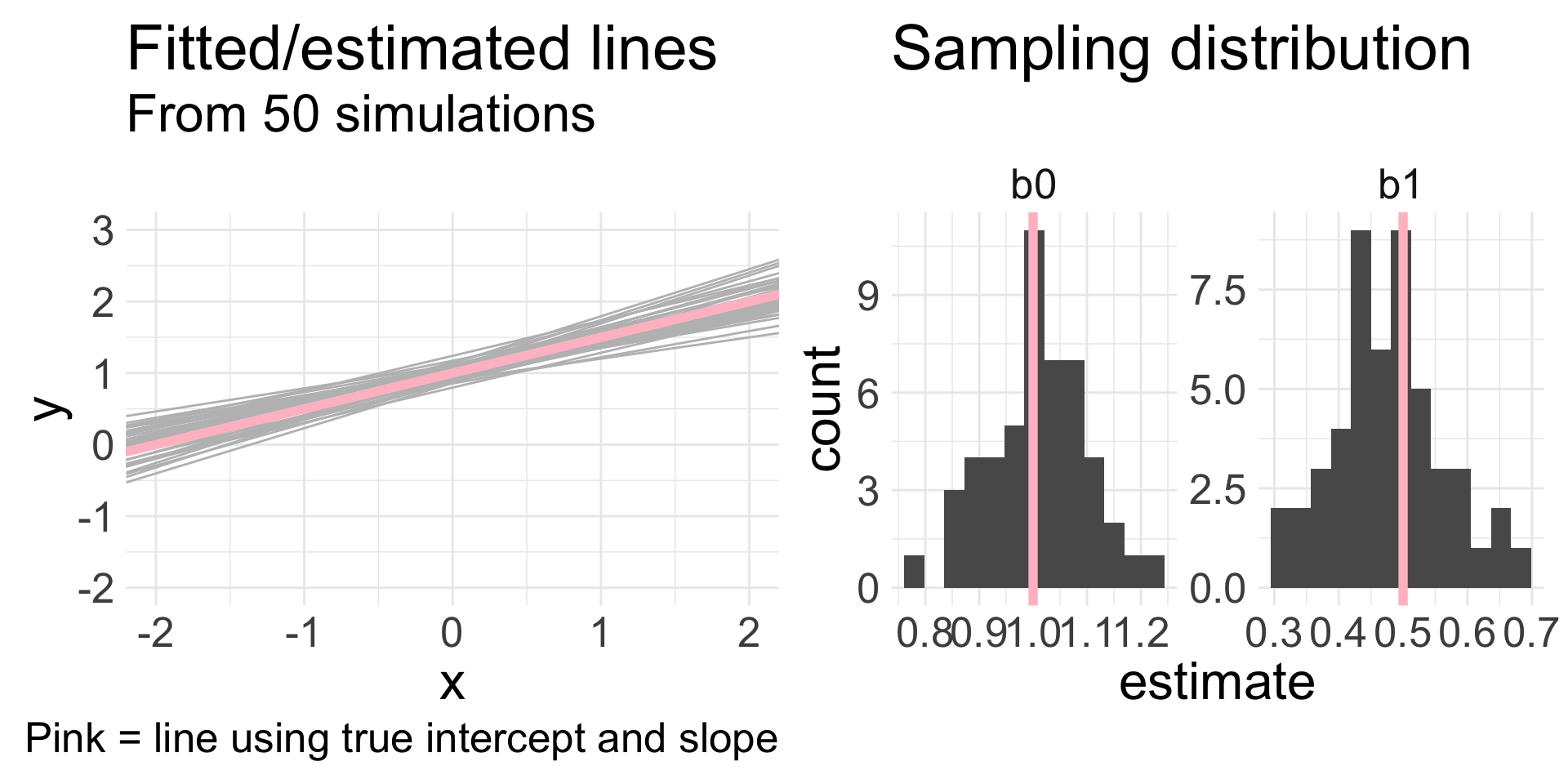
Variability of coefficient estimates
No need to take notes on this slide!
Remember, a linear regression is fit using a sample of data
Different samples from the same population will yield different point estimates of \((b_{0}, b_{1})\)
I will generate 30 data points under the following model: \(y = 1 + 0.5x+\epsilon\)
- How? Randomly generate some \(x\) and \(\epsilon\) values and then plug into model to get corresponding \(y\)
Fit SLR to these \((x,y)\) data, and obtain estimates \((b_{0}, b_{1})\)
Repeat this 50 times
Variability of coefficient estimates
What are we interested in?
Remember: we fit SLR to understand how \(x\) is (linearly) related to \(y\):
\[ y = \beta_{0} + \beta_{1} x + \epsilon \]
What would a value of \(\beta_{1} = 0\) mean?
- If \(\beta_{1} = 0\), then the effect of \(x\) disappears and there is in fact no linear relationship between \(x\) and \(y\)
We don’t know \(\beta_{1}\), so we can perform inference for it!
- Can conduct HTs and obtain CIs using our best guess \(b_{1}\)
Running example: evals data
Data on 463 courses at UT Austin were obtained to answer the question: “What factors explain differences in instructor teaching evaluation scores?”
One hypothesis is that attractiveness of a teacher influences their teaching evaluations
We will look at the variables:
score: course instructor’s average teaching score, where average is calculated from all students in that course. Scores ranged from 1-5, with 1 being lowest.bty_avg: course instructor’s average “beauty” score, where average is calculated from six student evaluations of “beauty”. Scores ranged from 1-10, with 1 being lowest.
Write out our linear regression model
Teaching evaluations data
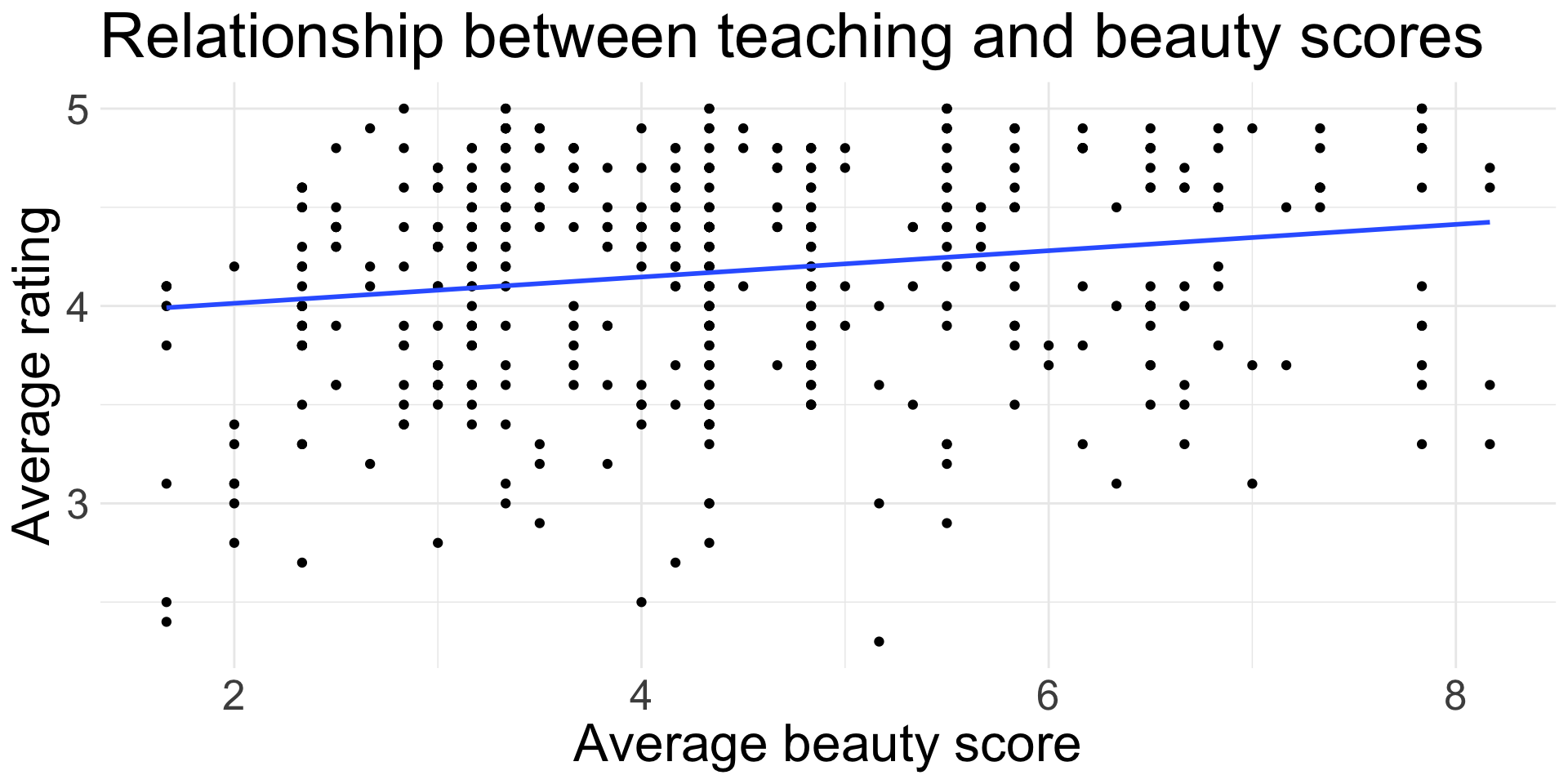
Does this line really have a non-zero slope?
Hypothesis test for slope
\(H_{0}: \beta_{1} = 0\): the true linear model has slope zero.
- In context: there is no linear relationship between an instructor’s average beauty score and their average teaching evaluation score.
\(H_{A}: \beta_{1} \neq 0\): the true linear model has a non-zero slope.
- In context: there is a linear relationship between an average instructor’s beauty score and average teaching evaluation score.
To assess, we do what we usually do:
Check if methods are appropriate
If so: obtain an estimate, identify/estimate standard error of the estimate, find an appropriate test statistic, and calculate p-value
The output from
lm()actually does all of #2 for us, but we will see how the test statistic and p-value are calculated!
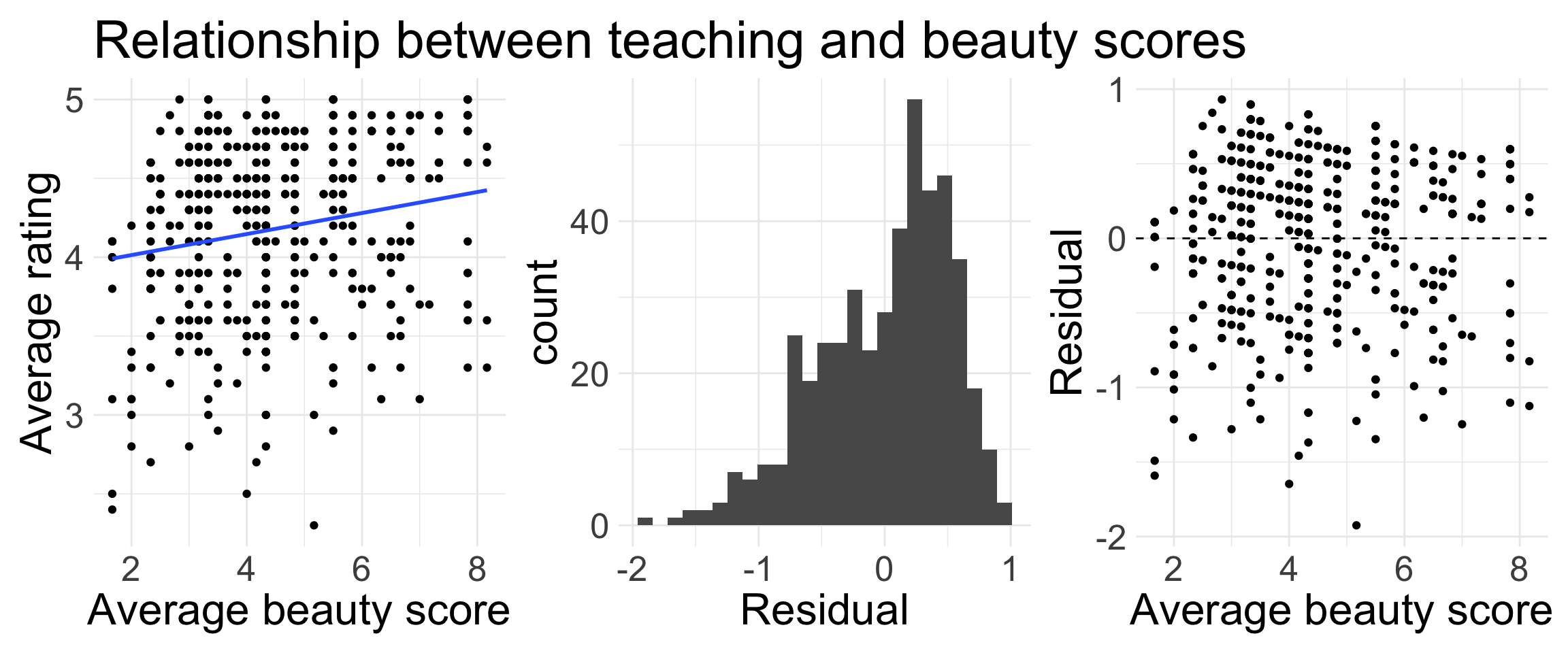
Teaching evaluations: model assessment
We fit the model in R, and obtain the following plots.
Are all conditions of LINE met?
Looking at lm() output
| term | estimate | std.error | statistic | p.value |
|---|---|---|---|---|
| (Intercept) | 3.880 | 0.076 | 50.961 | 0.00000 |
| bty_avg | 0.067 | 0.016 | 4.090 | 0.00005 |
Assuming the linear model is appropriate, interpret the coefficients!
Intercept: an instructor with an average beauty score of 0 has an estimated evaluation score of 3.88
Slope: for every one point increase in average beauty score an instructor receives, their evaluation score is estimated to increase by 0.067 points
Looking at lm() output
| term | estimate | std.error | statistic | p.value |
|---|---|---|---|---|
| (Intercept) | 3.880 | 0.076 | 50.961 | 0.00000 |
| bty_avg | 0.067 | 0.016 | 4.090 | 0.00005 |
estimate: point estimate (\(b_{0}\) or \(b_{1}\))std.error: estimated standard error of the estimate \((\widehat{\text{SE}})\)
statistic: value of the test statistic (follows \(t_{df = n-2}\) distribution for SLR)p.value: p-value associated with the two-sided alternative \(H_{A}: \beta_{1} \neq 0\)
- Let’s confirm the test statistic calculation:
\[ t = \frac{\text{observed} - \text{null}}{\widehat{\text{SE}_{0}}} =\frac{b_{1,obs} - \beta_{1, 0}}{\widehat{\text{SE}}_{0}} = \frac{0.067 - 0}{0.016} = 4.09 \]
p-value and conclusion
| term | estimate | std.error | statistic | p.value |
|---|---|---|---|---|
| (Intercept) | 3.880 | 0.076 | 50.961 | 0.00000 |
| bty_avg | 0.067 | 0.016 | 4.090 | 0.00005 |
Let’s confirm the p-value calculation:
\[\text{Pr}(T \geq 4.09) + \text{Pr}(T \leq -4.09) \qquad \text{ where } T \sim t_{461}\]
- Write out the code you would use to calculate the p-value.
2 * (1 - pt(4.09, df = 461))= 0.00005- Assuming the LINE conditions are met: since our p-value 0.00005 is extremely small, we would reject \(H_{0}\) at any reasonable significant level. Thus, the data provide convincing evidence that there is a linear relationship between instructor’s beauty score and evaluation score.
Different \(H_{A}\)
| term | estimate | std.error | statistic | p.value |
|---|---|---|---|---|
| (Intercept) | 3.880 | 0.076 | 50.961 | 0.00000 |
| bty_avg | 0.067 | 0.016 | 4.090 | 0.00005 |
Write code for your p-value if your alternative was \(H_{A}: \beta_{1} > 0\). What would your conclusion be?
\(\text{Pr}(T \geq 4.09)\) =
1-pt(4.09, 461)= 0.000025The data provide convincing evidence that there is a positive relationship between instructor’s beauty score and evaluation score.
Write code for your p-value if your alternative was \(H_{A}: \beta_{1} < 0\). What would your conclusion be?
\(\text{Pr}(T \leq 4.09)\) =
pt(4.09, 461)= 0.9999745The data do not provide convincing evidence that there is a negative relationship between instructor’s beauty score and evaluation score.
Confidence intervals
| term | estimate | std.error | statistic | p.value |
|---|---|---|---|---|
| (Intercept) | 3.880 | 0.076 | 50.961 | 0.00000 |
| bty_avg | 0.067 | 0.016 | 4.090 | 0.00005 |
We can also construct confidence intervals using the output from lm()! Remember:
\[ \text{CI} = \text{point est.} \pm \text{critical value} \times \widehat{\text{SE}} \qquad \text{ (or SE if we have it)} \]
Critical value also comes from \(t_{n-2}\) distribution
Suppose we want a 95% confidence intervals for \(\beta_{1}\):
What code would you use to obtain critical value? Then set up your CI!
qt(0.975, 461)= 1.97
\[\text{95% CI}: 0.067 \pm 1.97 \times 0.016 = (0.035, 0.099)\]
Remarks
Note: for \(\beta_{1}\), the null hypothesis is always of the form \(H_{0}: \beta_{1} = 0\)
LINE conditions must be met for underlying mathematical and probability theory to hold here! If not met, interpret and perform inference with caution
Here, the Independence and Normality conditions did not seem to be met
- Take STAT 412 or other course to learn how to incorporate dependencies between observations!
So what can we say?
The results suggested by our inference should be viewed as preliminary, and not conclusive
Further investigation is certainly warranted!
Checking LINE can be very subjective, but that’s how real-world analysis will be!